Object Detection

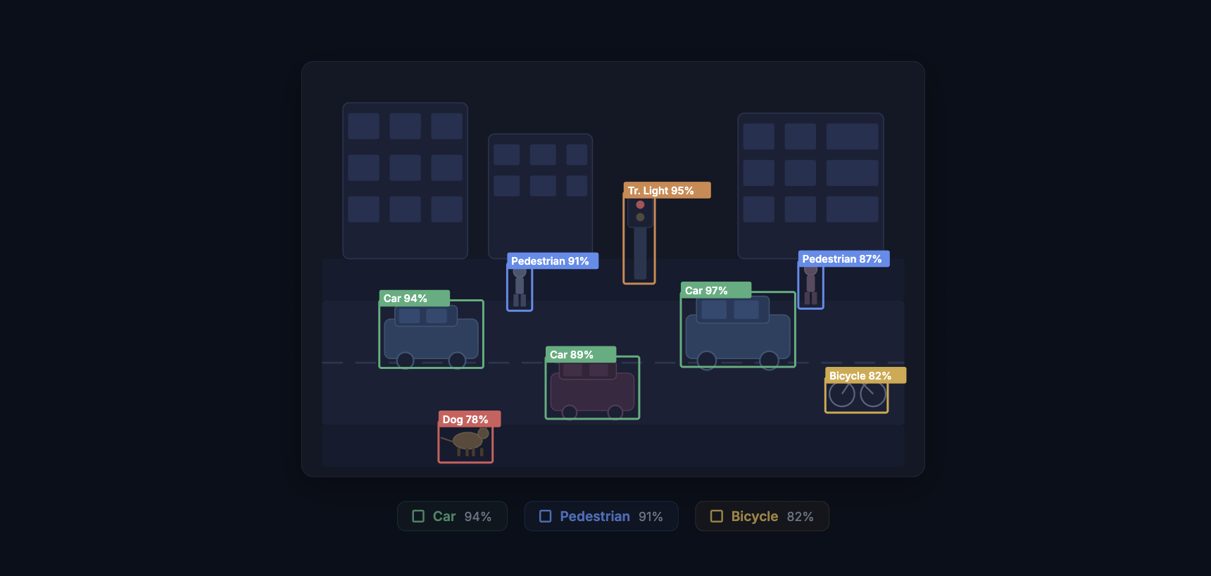
Object detection is the computer vision task of finding objects in an image and marking where each one sits. The model outputs a bounding box (a rectangle around the object) and a class label (what it is) for every instance it finds. A single image might contain dozens of objects from multiple categories, and a good detector will find them all, place tight boxes around each one, and assign the correct label with a confidence score.

This is different from image classification, which gives one label to the whole image. Detection answers two questions at once: "What objects are here?" and "Where exactly are they?" That pairing of recognition and localization is what makes object detection one of the most deployed tasks in production computer vision, from counting cars in satellite imagery to catching defective parts on a factory line.

How Object Detection Works

At a high level, every object detector does three things. It scans the image for regions that might contain objects. It extracts visual features from those regions. And it classifies each region while refining the bounding box coordinates. How those three steps are organized separates the major families of detectors.

Two-Stage Detectors

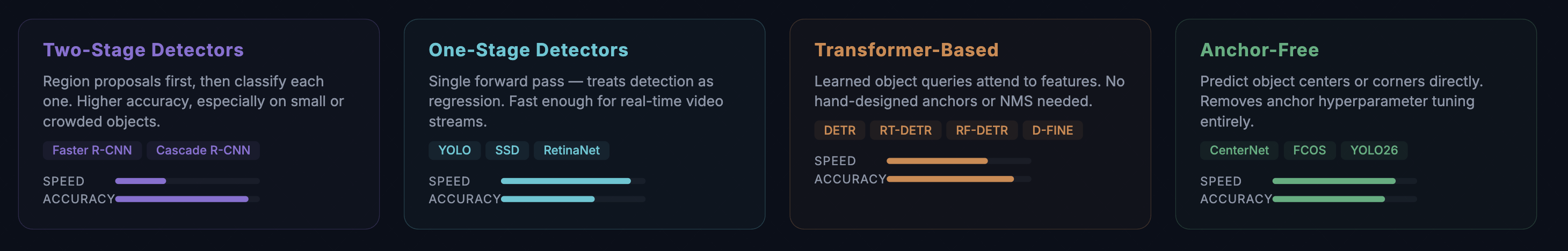
Two-stage detectors split the work into a proposal step and a classification step. The first stage generates candidate regions (region proposals) that are likely to contain objects. The second stage takes each proposal, extracts features using a backbone network like ResNet or ResNeXt, and predicts the class and refined box.

Faster R-CNN (2015) defined this family. Its Region Proposal Network (RPN) generates proposals directly inside the neural network rather than relying on a separate algorithm, which made the full pipeline trainable end-to-end. Cascade R-CNN stacks multiple detection heads with increasing IoU thresholds, progressively filtering out low-quality predictions. Two-stage detectors tend to deliver higher accuracy, especially on small objects and crowded scenes, but they run slower because of the two-pass architecture.

One-Stage Detectors

One-stage detectors skip the proposal step entirely. They divide the image into a grid (or set of anchor points) and predict bounding boxes and class probabilities for every cell in a single forward pass. This makes them much faster.

The YOLO (You Only Look Once) family is the most recognized example. The original YOLO paper in 2015 reframed detection as a regression problem: one pass through the network, one prediction grid, done. Each generation since then has pushed the speed-accuracy boundary further. YOLOv5 and YOLOv8 became community standards. YOLO11 introduced architectural refinements that improved small-object performance. YOLO26 (January 2026) shipped an NMS-free design with depthwise separable convolutions, cutting CPU inference time by 43% compared to its predecessor.

SSD (Single Shot MultiBox Detector) and RetinaNet also fall in the one-stage category. RetinaNet introduced focal loss, which down-weights easy examples during training and focuses the model on the hard-to-detect objects. This solved a persistent problem with one-stage detectors: they see far more background regions than object regions, and without focal loss, the flood of easy negatives drowns out the learning signal from actual objects.

Transformer-Based Detectors

DETR (Detection Transformer), published by Meta in 2020, replaced the entire hand-engineered post-processing pipeline with a transformer. It uses learned "object queries" (a fixed set of learnable embeddings) that attend to the image features and directly predict a set of detections. No anchor boxes. No non-maximum suppression. The Hungarian algorithm matches predictions to ground truth during training, and the model outputs a fixed-size set of predictions, most of which are "no object."

DETR was slow to converge and struggled with small objects. Deformable DETR fixed the convergence issue by using deformable attention (attending only to a small set of sampling points rather than the whole feature map). D-FINE pushed transformer detectors into real-time territory. RT-DETR and RF-DETR (2026) broke 60 AP on COCO, the first real-time models to reach that mark, combining transformer attention with efficient inference pipelines.

Anchor-Free Detectors

Anchor-based detectors pre-define a set of reference boxes at different scales and aspect ratios, then learn to adjust those anchors to fit actual objects. Anchor-free detectors remove this assumption. Instead, they predict objects by locating center points or corner points directly.

CenterNet predicts object centers as heatmap peaks and regresses width and height from those centers. FCOS (Fully Convolutional One-Stage) predicts distances from each pixel to the four sides of the bounding box. YOLO26 adopted an anchor-free approach, joining the broader trend away from hand-designed priors. Anchor-free methods simplify the pipeline and remove a source of hyperparameters (anchor sizes, aspect ratios, matching thresholds) that teams previously had to tune per dataset.

Key Metrics for Object Detection

Measuring detection performance is more involved than classification, because the model has to get both the label and the location right.

Intersection over Union (IoU) measures how much the predicted box overlaps with the ground truth box. It is the area of overlap divided by the area of union. An IoU of 1.0 means a perfect match. Most benchmarks consider a detection correct if its IoU exceeds a threshold, typically 0.50.

Precision is the fraction of the model's detections that are correct. Recall is the fraction of ground-truth objects that the model found. The precision-recall curve shows the tradeoff across confidence thresholds.

Average Precision (AP) summarizes the precision-recall curve into a single number by computing the area under the curve for one class. Mean Average Precision (mAP) averages AP across all classes. The COCO benchmark reports mAP at IoU thresholds from 0.50 to 0.95 in steps of 0.05 (written as mAP@[.50:.95]), which is more demanding than mAP@0.50 alone because it penalizes loose bounding boxes.

COCO also breaks down AP by object size: AP-small (objects under 32x32 pixels), AP-medium (32x32 to 96x96), and AP-large (above 96x96). This matters because small-object detection is one of the hardest unsolved problems in the field, and aggregate mAP numbers can hide poor performance on small objects.

Training an Object Detection Model

Training a detector follows the same general loop as any supervised learning task, but with a few detection-specific steps.

Data collection. Gather images that match the conditions your model will see in production. Vary the lighting, camera angles, backgrounds, and object density. If you are building a defect detector for a production line, collect images from every shift, every product variant, and every lighting condition. Models trained on one set of conditions fail when conditions change.

Annotation. Every object in every image needs a bounding box and a class label. For a 5,000-image dataset with an average of 8 objects per image, that is 40,000 individual annotations. This is the bottleneck. AI-assisted annotation tools, model-assisted labeling, and active learning all help reduce the effort. Consensus algorithms catch labeling errors by comparing annotations from multiple labelers.

Data augmentation. Image augmentation artificially expands the training set. Random horizontal flips, rotations, scaling, color jitter, and mosaic transforms (stitching four images together) help the model generalize. Mosaic augmentation, introduced in YOLOv4, is especially effective for detection because it exposes the model to objects at different scales and contexts within every training batch.

Transfer learning. Starting from a pre-trained backbone (a model trained on ImageNet, COCO, or Objects365) gives the network strong low-level features from day one. You fine-tune the detector on your specific dataset, which saves time and typically produces better results than training from scratch, especially with limited data. For a full walkthrough, see our guide to training a YOLOv8 detection model on a custom dataset.

Evaluation. Split the data into training, validation, and test sets. Monitor training graphs for loss convergence, overfitting (validation loss diverging from training loss), and learning rate scheduling. Evaluate final performance with mAP on the held-out test set.

Common Challenges

Small object detection. Objects that occupy fewer than 32x32 pixels in the image are hard to detect because they contain very little visual information after downsampling through the network. SAHI (Slicing Aided Hyper Inference) addresses this by running detection on overlapping crops of the full image, then merging results. Feature Pyramid Networks (FPN) and multi-scale feature fusion also improve small-object accuracy by preserving high-resolution features deeper into the network.

Occlusion. When objects overlap or partially hide behind other objects, detectors can miss them or merge two objects into one box. Two-stage detectors handle occlusion better than most one-stage detectors because the proposal mechanism gives each candidate region its own classification pass.

Class imbalance. Most pixels in most images are background. In a dataset of shelf images, the model sees background a hundred times more often than any specific product. Focal loss, hard negative mining, and oversampling rare classes help the model learn from the minority classes.

Domain shift. A detector trained on well-lit studio photos will underperform on grainy security camera footage. The visual statistics are different. Fine-tuning on in-domain data, domain randomization during training, and test-time augmentation all reduce the gap.

Real-World Applications

Manufacturing quality inspection. Detecting scratches, dents, missing components, and assembly errors on a production line. Automated visual inspection runs at line speed, catches defects that human inspectors miss during long shifts, and generates traceable records. Companies like Ingroth use detection models to inspect industrial barrels and Trendspek uses them to find structural cracks in infrastructure.

Autonomous vehicles. Self-driving cars run multiple detection models simultaneously: one for pedestrians and cyclists, one for vehicles and traffic signs, one for lane markings and road edges. Latency matters here. The system must process a new frame every 30 to 100 milliseconds, which is why YOLO-class models dominate this space.

Medical imaging. Detecting nodules in lung CT scans, lesions on skin photographs, polyps in colonoscopy video, and fractures in X-rays. Medical detection models do not replace radiologists. They flag suspicious regions for human review, reducing the chance that something gets missed in a stack of hundreds of images.

Retail and inventory. Counting products on shelves, verifying planogram compliance (are products in the right position?), and powering checkout-free stores where cameras track which items shoppers pick up and put back.

Agriculture. Counting fruit on trees for yield estimation, detecting weeds among crops for precision herbicide application, and grading produce quality on sorting lines. Drone-mounted cameras cover large fields fast, and edge-deployed models process images without cloud connectivity.

Security and surveillance. Detecting people in restricted zones, identifying unattended bags, counting foot traffic, and reading license plates at parking lot entrances.

Object Detection vs. Related Tasks

Detection is one of several related but distinct computer vision tasks. Knowing which one to use matters.

Classification assigns one label to the whole image. Use it when you only need to know "what is this?" and the image contains one dominant subject (pass/fail sorting, X-ray screening).

Object detection finds multiple objects and marks their bounding boxes. Use it when you need to count objects, locate them, or track their positions.

Instance segmentation goes a step further and draws a pixel-level mask around each object instead of a rectangle. Use it when precise boundaries matter (measuring the area of a defect, segmenting overlapping cells in a microscope image). See our guide to training an instance segmentation model for a hands-on walkthrough.

Object tracking extends detection into video by assigning persistent IDs to objects across frames. A detector runs on each frame, and a tracking algorithm matches detections over time. Use it for counting unique objects passing a line, analyzing movement patterns, or measuring speed.

Deploying Object Detection Models

A trained model is only useful once it runs in its target environment. Deployment adds constraints that training does not: latency budgets, memory limits, and reliability requirements.

Cloud deployment wraps the model in an API endpoint. Input images go up, predictions come back. This works when latency tolerance is in the hundreds of milliseconds and the client has a reliable internet connection.

Edge deployment runs the model on local hardware: NVIDIA Jetson for industrial settings, Raspberry Pi for lightweight applications, or mobile SoCs for phone-based detection. Edge deployment eliminates network latency and keeps sensitive data on-premises.

Model optimization techniques make deployment practical. Post-training quantization reduces model weights from 32-bit floats to 8-bit integers, cutting model size by 4x and speeding up inference on hardware that supports integer math. Model pruning removes redundant weights and neurons, shrinking the model further. TensorRT, ONNX Runtime, and TFLite each optimize inference for their target hardware.

Getting Started with Object Detection

The fastest path to a working detector is to pick a pre-trained model and fine-tune it on your data. The YOLO family offers the widest range of model sizes (from YOLO-Nano for edge devices to YOLO-XL for maximum accuracy) and the most active community support. For accuracy-first applications where inference speed is less critical, a transformer-based detector like RT-DETR or D-FINE is worth benchmarking.

Datature Nexus handles the full detection pipeline in a single platform: upload images, draw bounding boxes with AI-assisted annotation, train a YOLO or EfficientDet model, evaluate results with built-in metrics, and deploy to cloud or edge. No infrastructure code required. Visit the Datature Blog for deeper guides on every topic covered here.