OpenCV Functions Every Computer Vision Engineer Should Know

OpenCV Functions Every Computer Vision Engineer Should Know

Most OpenCV tutorials start with imread and imshow. Fair enough. But those two functions get you to "I can load a picture." They do not get you to "I can build something useful."

These seven functions do. They cover the core operations that appear across production computer vision work: running neural networks, correcting geometry, tracking motion, separating foreground from background, finding object outlines, detecting edges, and filtering by color. We ran each one on real images so you can see the input, the code, and the output side by side.

All code runs with OpenCV 4.x and Python 3. No GPU needed.

1. dnn.readNet + blobFromImage: Neural Network Inference

OpenCV ships with its own deep learning inference engine. You can load models trained in Caffe, TensorFlow, ONNX, or Darknet and run them with zero framework dependencies. No torch.load(), no TensorFlow session. Just OpenCV.

This is useful when you need to deploy a pre-trained model on a machine where installing PyTorch or TensorFlow is not practical. Think embedded systems, locked-down servers, or quick prototypes where pulling in a 2 GB framework is overkill.

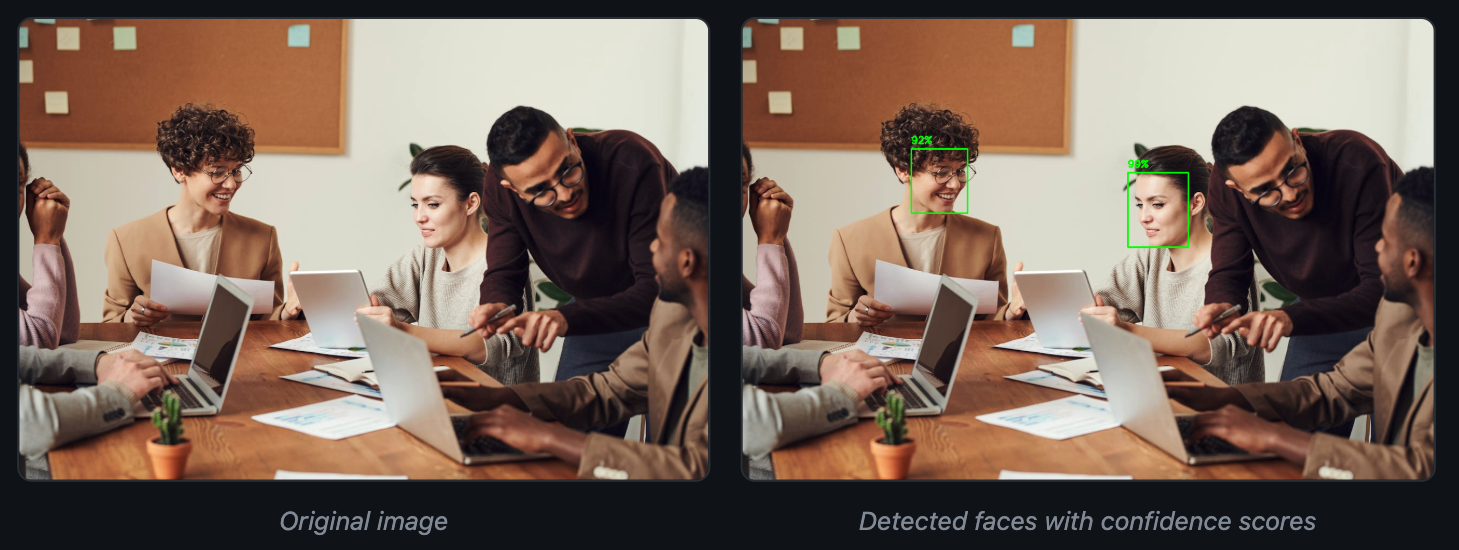
Here is face detection using a pre-trained Caffe model:

import cv2
import numpy as np

img = cv2.imread("office_people.jpg")
net = cv2.dnn.readNetFromCaffe("face_deploy.prototxt", "face_detect.caffemodel")

h, w = img.shape[:2]
blob = cv2.dnn.blobFromImage(
    cv2.resize(img, (300, 300)), 1.0, (300, 300), (104.0, 177.0, 123.0)
)
net.setInput(blob)
detections = net.forward()

result = img.copy()
for i in range(detections.shape[2]):
    confidence = detections[0, 0, i, 2]
    if confidence > 0.5:
        box = detections[0, 0, i, 3:7] * np.array([w, h, w, h])
        x1, y1, x2, y2 = box.astype("int")
        cv2.rectangle(result, (x1, y1), (x2, y2), (0, 255, 0), 2)
        cv2.putText(result, f"{confidence:.0%}", (x1, y1 - 10),
                    cv2.FONT_HERSHEY_SIMPLEX, 0.6, (0, 255, 0), 2)

blobFromImage handles resizing, mean subtraction, and conversion to the 4D blob format that neural networks expect (batch, channels, height, width). The scalefactor 1.0 means no pixel scaling (this particular Caffe model handles normalization internally; other models may use 1/255.0 or 1/127.5). The mean values (104.0, 177.0, 123.0) come from the model's training data.

OpenCV's DNN module supports most common architectures out of the box. You can load ONNX models exported from PyTorch, frozen TensorFlow graphs, Darknet configs (YOLO), and Caffe models. For a deep look at how detection models like YOLO have evolved over the past decade, see our historical breakdown.

2. warpPerspective: Perspective Correction

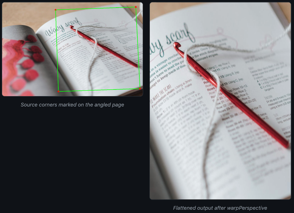
Cameras rarely look straight down at the thing you care about. Documents tilt. License plates sit at angles. Conveyor belt items shift under the lens. warpPerspective takes a skewed view and maps it to a flat, rectangular output.

You give it four points on the source image (the corners of the region you want to straighten) and four points defining where those corners should land in the output. OpenCV computes the 3x3 transformation matrix and warps every pixel.

import cv2
import numpy as np

img = cv2.imread("receipt_angle.jpg")
h, w = img.shape[:2]

# Four corners of the page in the original (skewed) image
src_pts = np.float32([
    [w * 0.38, h * 0.08],   # top-left
    [w * 0.95, h * 0.05],   # top-right
    [w * 0.98, h * 0.92],   # bottom-right
    [w * 0.40, h * 0.95],   # bottom-left
])

# Where those corners should end up
dst_pts = np.float32([[0, 0], [500, 0], [500, 700], [0, 700]])

M = cv2.getPerspectiveTransform(src_pts, dst_pts)
warped = cv2.warpPerspective(img, M, (500, 700))

‍

The hard part is finding those four corner points automatically. For documents on clean backgrounds, contour detection (see function #5) finds them well. For messier scenes, you might need edge detection plus Hough line intersection, or a trained corner-prediction model.

Document scanning apps, automated receipt processing, and industrial part alignment all depend on this function.

3. calcOpticalFlowPyrLK: Sparse Optical Flow

Video is where OpenCV gets interesting. calcOpticalFlowPyrLK tracks how individual pixels move between two consecutive frames. It uses the Lucas-Kanade method with image pyramids, which means it handles both small and large displacements.

The pattern: detect good feature points in frame 1 with goodFeaturesToTrack, then pass both frames to calcOpticalFlowPyrLK to find where each point ended up.

import cv2
import numpy as np

frame1 = cv2.imread("frame1.jpg")
frame2 = cv2.imread("frame2.jpg")

gray1 = cv2.cvtColor(frame1, cv2.COLOR_BGR2GRAY)
gray2 = cv2.cvtColor(frame2, cv2.COLOR_BGR2GRAY)

# Find strong corners in the first frame
corners = cv2.goodFeaturesToTrack(
    gray1, maxCorners=200, qualityLevel=0.01, minDistance=20
)

# Track them into the second frame
new_pts, status, err = cv2.calcOpticalFlowPyrLK(gray1, gray2, corners, None)

# Draw flow arrows
for i, (new, old) in enumerate(zip(new_pts, corners)):
    if status[i] == 1:
        a, b = new.ravel().astype(int)
        c, d = old.ravel().astype(int)
        cv2.arrowedLine(frame1, (c, d), (a, b), (0, 255, 0), 2, tipLength=0.3)

‍

Each green arrow shows the direction and magnitude of movement for one tracked point. The status array tells you which points were tracked successfully and which were lost (due to occlusion, leaving the frame, or insufficient texture).

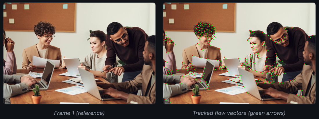
For this demo we simulated motion by shifting the image 15 pixels right and 8 pixels down. On real video, you will see varying flow directions across the frame as different objects move independently. Uniform arrows like these confirm the tracker is working; in practice the flow field is far more varied and informative.

Optical flow is the foundation of video stabilization, object tracking, action recognition, and drone navigation. When you need to know "how fast is this thing moving and in which direction," optical flow gives you per-pixel answers, frame by frame.

4. createBackgroundSubtractorMOG2: Background Subtraction

Security cameras, traffic monitors, and factory line cameras all share one problem: the background stays roughly the same while the interesting stuff (people, cars, products) moves through the scene. Background subtraction builds a statistical model of what "normal" looks like, then flags anything that deviates.

MOG2 (Mixture of Gaussians, version 2) models each pixel as a mixture of Gaussian distributions. It learns the background over time and adapts to gradual changes like shifting sunlight or swaying branches.

import cv2
import numpy as np

mog2 = cv2.createBackgroundSubtractorMOG2(
    history=50, varThreshold=50, detectShadows=True
)

cap = cv2.VideoCapture("factory_feed.mp4")
while cap.isOpened():
    ret, frame = cap.read()
    if not ret:
        break

    # Returns a mask: 0=background, 127=shadow, 255=foreground
    mask = mog2.apply(frame)

    # Clean up with morphological opening
    kernel = cv2.getStructuringElement(cv2.MORPH_ELLIPSE, (5, 5))
    mask = cv2.morphologyEx(mask, cv2.MORPH_OPEN, kernel)

‍

We used a synthetic scene for this demo (a moving rectangle on a gradient background). On a real camera feed, MOG2 produces the same kind of clean foreground masks for people, vehicles, or products passing through the frame.

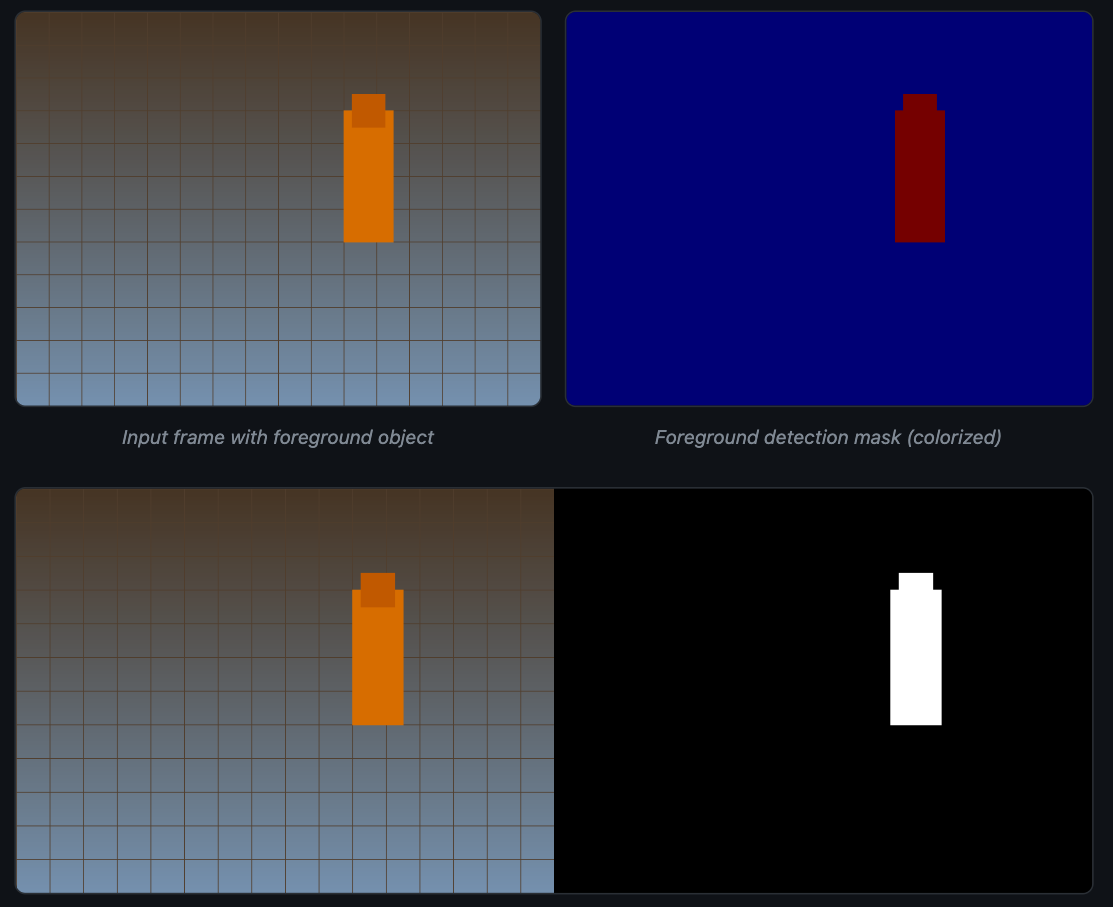
The white regions in the mask represent pixels MOG2 classified as foreground. Shadows appear as gray (value 127) when detectShadows=True, which helps you separate actual objects from the shadows they cast.

history controls how many recent frames the model remembers. A short history (50 frames) adapts fast but may absorb slow-moving objects into the background. A long history (500+ frames) takes longer to learn but stays more stable. varThreshold sets how sensitive the detector is to change.

5. findContours: Shape Detection and Measurement

Once you have a binary image (from edge detection, thresholding, or background subtraction), findContours extracts the boundaries of every white region. Each contour is a list of (x, y) coordinates that trace the outline of one connected shape.

The power comes from what you can do after extraction. OpenCV provides functions to compute area, perimeter, bounding rectangles, centroids, and shape approximations for each contour. That turns raw pixels into measurements you can act on.

import cv2

img = cv2.imread("gears.jpg")
gray = cv2.cvtColor(img, cv2.COLOR_BGR2GRAY)
blurred = cv2.GaussianBlur(gray, (5, 5), 0)
edges = cv2.Canny(blurred, 30, 100)

contours, hierarchy = cv2.findContours(
    edges, cv2.RETR_EXTERNAL, cv2.CHAIN_APPROX_SIMPLE
)

result = img.copy()
for cnt in contours:
    area = cv2.contourArea(cnt)
    if area > 500:  # Skip tiny noise contours
        cv2.drawContours(result, [cnt], -1, (0, 255, 0), 2)
        M = cv2.moments(cnt)
        cx = int(M["m10"] / M["m00"])
        cy = int(M["m01"] / M["m00"])
        cv2.putText(result, f"{area:.0f}px", (cx - 30, cy),
                    cv2.FONT_HERSHEY_SIMPLEX, 0.5, (255, 255, 0), 2)

‍

RETR_EXTERNAL tells OpenCV to return only the outermost boundaries, ignoring any holes or nested shapes inside. CHAIN_APPROX_SIMPLE compresses straight segments down to their endpoints, which saves memory without losing shape accuracy.

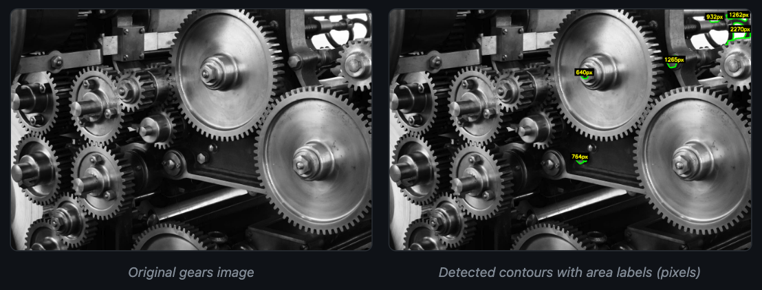
Quality inspection teams use contour analysis to measure parts on a production line and flag deviations. Count objects on a conveyor belt, measure the diameter of a bearing, check whether a gasket matches the template. All of that flows from findContours and a few lines of geometry. For teams building these pipelines, image augmentation during training helps models generalize across varying lighting and part orientations.

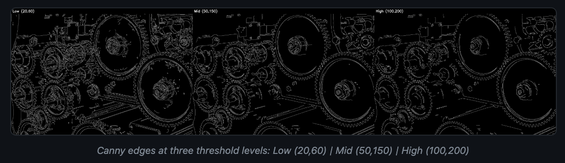
6. Canny: Edge Detection

John Canny published this algorithm in 1986. Forty years later, it is still the default edge detector in most OpenCV code. The function takes a grayscale image and returns a binary map where white pixels mark sharp intensity transitions.

It works in four stages: Gaussian smoothing, gradient computation with Sobel filters, non-maximum suppression to thin edges to one pixel wide, and hysteresis thresholding with two values (low and high) to keep real edges and discard noise.

import cv2

img = cv2.imread("gears.jpg")
gray = cv2.cvtColor(img, cv2.COLOR_BGR2GRAY)
blurred = cv2.GaussianBlur(gray, (5, 5), 0)

edges_low = cv2.Canny(blurred, 20, 60)     # Sensitive
edges_mid = cv2.Canny(blurred, 50, 150)    # Balanced
edges_high = cv2.Canny(blurred, 100, 200)  # Conservative

‍

Low thresholds catch more edges but also pick up noise and texture you probably do not want. High thresholds give clean outlines but miss faint or low-contrast boundaries. A ratio between 1:2 and 1:3 for the low and high thresholds is a reliable starting point (50 and 150, or 50 and 100).

For automated threshold selection, compute them from the image median:

import numpy as np

median = np.median(blurred)
lower = int(max(0, 0.7 * median))
upper = int(min(255, 1.3 * median))
edges = cv2.Canny(blurred, lower, upper)

Canny is the standard first step before contour detection, line detection (HoughLinesP), and many shape analysis workflows. It pairs well with deep learning too: some teams run Canny as a fast filter to identify regions of interest, then send only those crops to a heavier model for classification.

7. inRange + morphologyEx: Color-Based Segmentation

Color filtering sounds simple until you try it in RGB. Lighting changes, shadows, and white balance shifts make RGB thresholds break constantly. Switch to HSV (Hue, Saturation, Value) and the problem gets much easier, because hue stays roughly stable regardless of brightness.

inRange creates a binary mask where pixels within a given color range are white and everything else is black. morphologyEx then cleans up that mask by closing small holes and removing stray noise pixels.

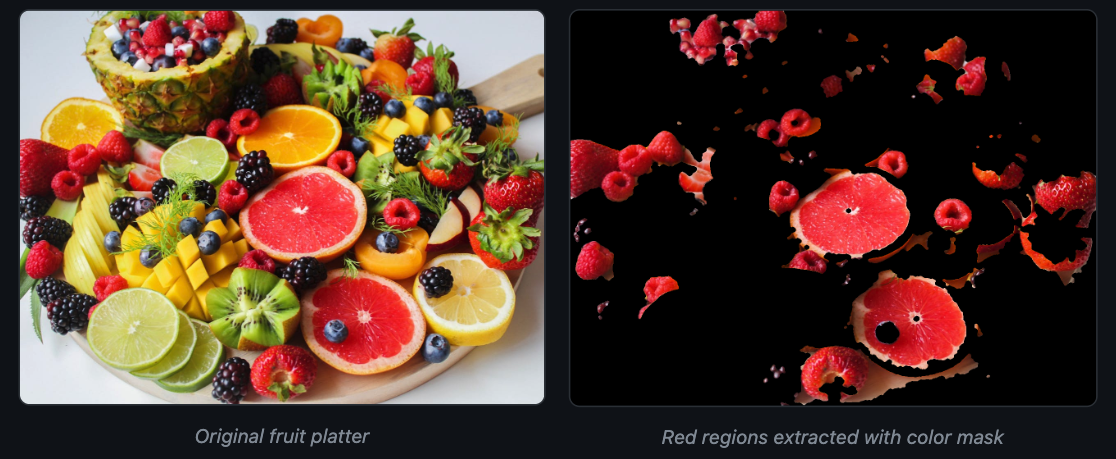
import cv2
import numpy as np

img = cv2.imread("colorful_fruits.jpg")
hsv = cv2.cvtColor(img, cv2.COLOR_BGR2HSV)

# Red wraps around the hue circle, so we need two ranges
lower_red1, upper_red1 = np.array([0, 80, 80]), np.array([10, 255, 255])
lower_red2, upper_red2 = np.array([160, 80, 80]), np.array([180, 255, 255])

mask1 = cv2.inRange(hsv, lower_red1, upper_red1)
mask2 = cv2.inRange(hsv, lower_red2, upper_red2)
raw_mask = mask1 | mask2

# Morphological cleanup
kernel = cv2.getStructuringElement(cv2.MORPH_ELLIPSE, (7, 7))
cleaned = cv2.morphologyEx(raw_mask, cv2.MORPH_CLOSE, kernel, iterations=2)
cleaned = cv2.morphologyEx(cleaned, cv2.MORPH_OPEN, kernel, iterations=1)

# Apply mask to original
result = cv2.bitwise_and(img, img, mask=cleaned)

‍

The raw mask has holes inside the red regions and speckles outside them. MORPH_CLOSE (dilation then erosion) fills the holes. MORPH_OPEN (erosion then dilation) removes the speckles. Two operations, and the mask goes from noisy to usable.

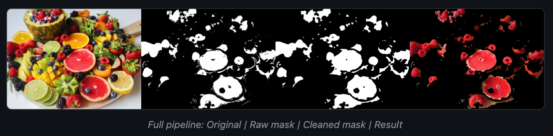
Red is a special case in HSV because hue wraps around at 180 (OpenCV uses 0-180 for hue, not 0-360). Most other colors (blue, green, yellow) need only a single range. For production systems where lighting varies between shifts, calibrating these thresholds on a reference color target at startup keeps accuracy high.

Color filtering shows up in fruit sorting, safety equipment detection (spotting yellow hard hats), and industrial inspection (isolating colored components on a circuit board).

Tying These Together

Most production pipelines chain two or three of these together. Canny feeds into findContours. Background subtraction feeds into contour analysis for object counting. Color filtering feeds into contour measurement for defect sizing.

Even as deep learning models take on more of the heavy lifting, OpenCV stays in the loop. You use it to preprocess frames before inference, draw predictions back onto the image, and post-process model outputs into actionable measurements. For teams deploying to edge devices like Raspberry Pi, OpenCV is often the only image processing library on the device.

If you want to build computer vision systems without writing model training and deployment infrastructure from scratch, Datature Nexus handles labeling, training, and deployment through a visual interface. OpenCV handles the image plumbing. Datature handles the ML plumbing.