How to Annotate DICOM Images for Medical Image Segmentation

TL;DR

• Medical image annotation is the bottleneck. A single CT volume takes 30-90 minutes to segment by hand, and most segmentation projects need hundreds of annotated volumes. The tooling you pick determines whether this stage takes weeks or months.
• DICOM is not JPEG. Any annotation tool you evaluate must parse DICOM headers, reconstruct 3D volumes, render multi-planar views (axial, sagittal, coronal), and handle Hounsfield unit windowing. Generic 2D platforms fail here.
• No single tool wins everywhere. 3D Slicer is the gold standard for solo research. Cloud platforms like Datature close the gaps around team collaboration, SAM-assisted DICOM annotation, and integrated training. Pick the tool that matches your team size, your data volume, and whether you need a training pipeline downstream.

Why Medical Image Annotation Is the Bottleneck

Every medical image segmentation paper describes model architectures, loss functions, and DICE scores. Few describe how the training data was produced. That silence hides the hardest part of the entire pipeline.

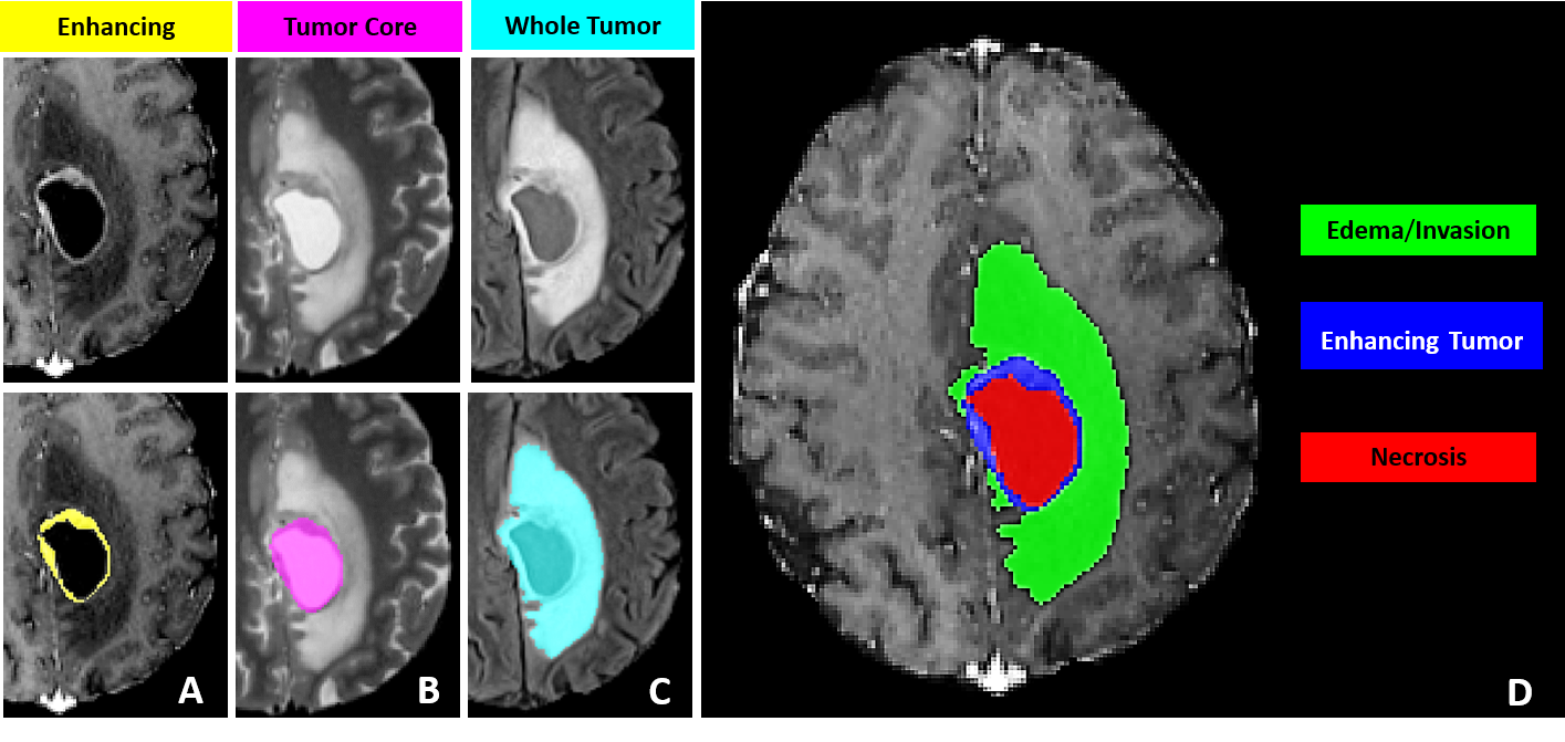
Consider brain tumor segmentation. The BraTS challenge requires annotators to delineate three tumor sub-regions (enhancing tumor, necrotic core, peritumoral edema) across four MRI sequences (T1, T1ce, T2, FLAIR) for every patient volume. A trained neuroradiologist needs 30 to 60 minutes per scan. A dataset of 1,000 volumes, which is modest by current standards, demands thousands of hours of expert annotation. Finding radiologists with free time is a problem that no model architecture can solve.

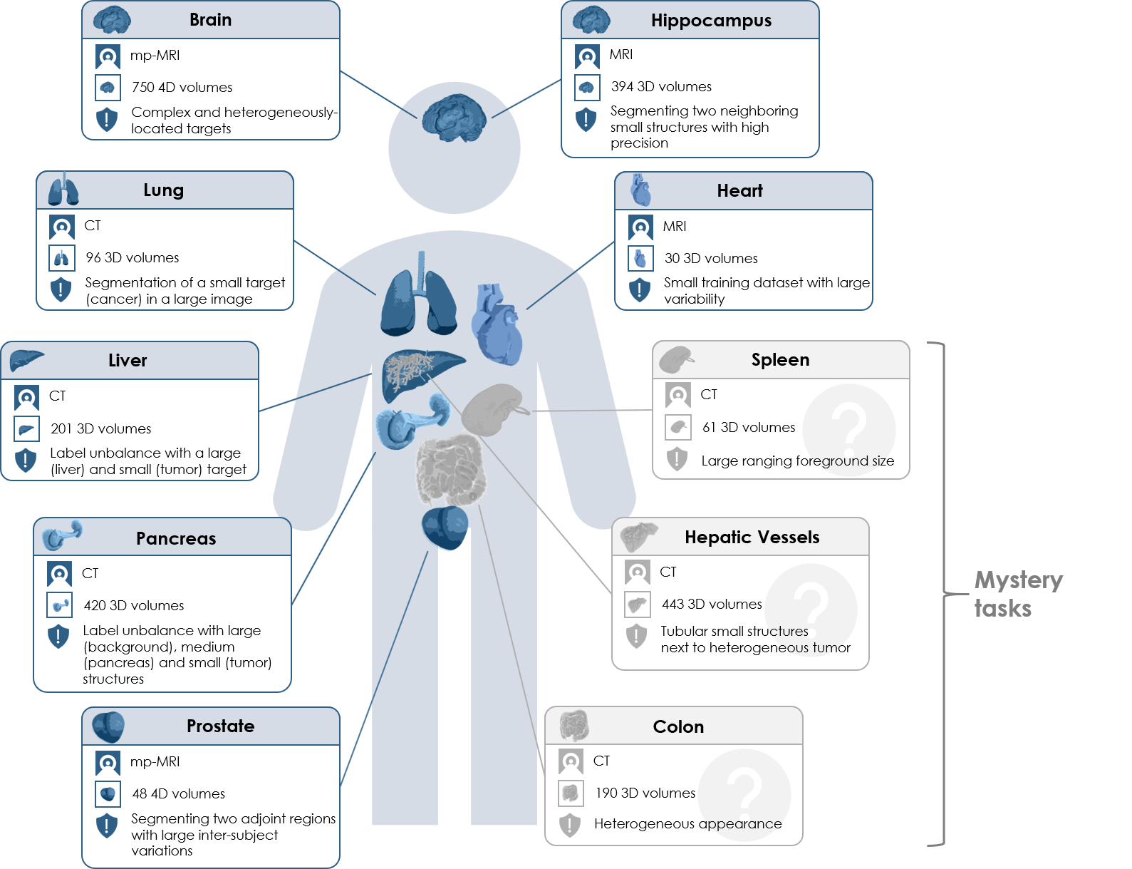
The arithmetic gets worse for multi-organ segmentation. The AMOS benchmark covers 15 abdominal organs across CT and MRI. The Medical Segmentation Decathlon spans 10 tasks across different organs and modalities. Each of these datasets represents a massive annotation investment before a single training run begins.

This is why annotation tooling matters so much. The difference between a tool that takes 45 minutes per volume and one that takes 15 minutes (through AI-assisted pre-segmentation and efficient multi-planar navigation) is the difference between a project that ships in three months and one that stalls for a year.

What Makes DICOM Annotation Different

If your experience with annotation comes from labeling natural images (bounding boxes on photos, polygon masks on satellite imagery), medical imaging will feel like a different discipline. It is.

DICOM (Digital Imaging and Communications in Medicine) is the universal file format for clinical imaging. A single CT scan is not one image file. It is a folder containing hundreds of .dcm files, each representing one 2D slice. Each file carries a metadata header with patient information, scanner parameters, pixel spacing, and slice thickness. A full chest CT might contain 300 to 500 slices at 512 x 512 resolution, and the annotation tool must reconstruct them into a coherent 3D volume.

Three properties separate DICOM annotation from natural-image annotation:

Multi-planar reconstruction (MPR). Radiologists move between three orthogonal planes: axial (top-down), sagittal (side), and coronal (front). An annotation that looks correct on the axial slice may have ragged edges in the sagittal view. Any serious medical annotation tool must render all three planes.

Hounsfield unit (HU) windowing. CT pixel values are measured in Hounsfield units, where air is -1000 HU, water is 0 HU, and dense bone reaches +1000 HU or higher. A lung window (center -600, width 1500) reveals airway structures invisible in a soft-tissue window (center 40, width 400). The annotator needs to switch presets to see different anatomical structures. Tools that only display raw pixel intensity will not work.

Volumetric masks. In natural image annotation, a mask is a 2D pixel array. In medical imaging, it is a 3D voxel array. Each voxel maps to a physical location with known x, y, and z spacing. The annotation tool must track spatial consistency across slices, and exported masks must preserve voxel spacing and orientation for training to produce correct results.

For a glossary-level introduction to the task itself, see our entry on semantic segmentation. The concepts (per-pixel class assignment, mask generation) are the same in 2D and 3D, but the tooling requirements diverge sharply once volumetric data enters the picture.

The Tool Landscape: An Honest Comparison

There are more medical annotation tools than you might expect, and they fall into two camps: desktop research tools with deep functionality and long histories, and cloud platforms built for team-scale annotation with newer medical imaging support. Both camps have strengths. Neither camp covers everything.

Desktop Research Tools

3D Slicer is the gold standard for academic medical image analysis. Free, open source, and backed by 20+ years of development. The Segment Editor supports manual painting, threshold-based segmentation, level tracing, and dozens of specialized extensions through a plugin ecosystem with 500+ community modules. If you are a solo researcher or a small lab, 3D Slicer is the correct starting point. The weakness: it is a desktop application with no built-in team workflows, no annotation versioning, and no cloud sync. Scaling from one annotator to ten means managing ten independent copies of the data.

ITK-SNAP is lighter and faster than 3D Slicer for a specific task: carving out a single 3D region of interest using active contour (snake) segmentation. Radiologists who need to delineate one structure quickly often prefer it. But it historically handles one label at a time (recent versions have added multi-label support), has no AI-assisted tools, and offers no team features.

MONAI Label runs as a server that plugs into 3D Slicer (or OHIF Viewer). It adds AI-assisted annotation through an active learning loop: annotate a few volumes, train a model, use it to pre-segment the next batch, correct, retrain. The concept is powerful. The setup is not trivial: local NVIDIA GPU, Python environment with the MONAI stack, and server-client configuration. Works well for a lab with an ML engineer on staff. Does not work for a team of radiologists who want to open a browser and start annotating.

Cloud Annotation Platforms

MD.ai is purpose-built for radiology. It handles DICOM natively, runs in the browser, and has a strong community in academic medical imaging research. The limitation: MD.ai stops at annotation. Moving masks into a training pipeline is a separate process.

Encord and V7 are general-purpose enterprise annotation platforms that have added medical imaging support. Both offer team management, QA workflows, and AI-assisted labeling. Their DICOM support has improved but is not their core focus.

Datature occupies a specific niche: cloud-native DICOM support with MPR viewing, manual annotation, SAM-based interactive segmentation on DICOM slices, and model-assisted tools, plus team collaboration with consensus workflows and a built-in training pipeline that goes from annotated volumes to a deployed segmentation model without exporting data to a separate system. The honest tradeoff: Datature uses general SAM (not a medical-fine-tuned variant like MedSAM), does not have 3D Slicer's plugin ecosystem, and lacks MONAI Label's domain-specific pre-trained models. We cover the specific strengths and weaknesses in Section 10.

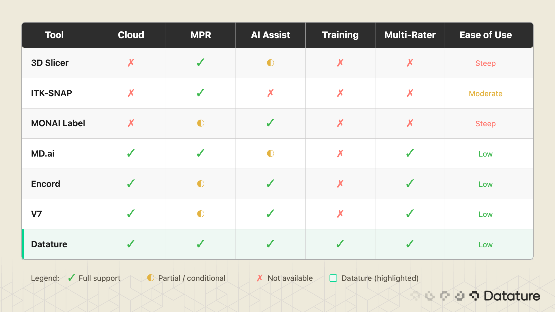
The table above is not a ranking. It is a feature map. A solo PhD student running 3D Slicer with MONAI Label has a perfectly valid setup. A 10-person annotation team at a healthtech startup building an FDA-submission dataset needs something different. Know your constraints before picking a tool.

The DICOM-to-Trained-Model Workflow

Regardless of which tool you use, the workflow from raw DICOM to a trained segmentation model follows the same steps. The pipeline has nine stages:

1. Acquire DICOM data from a hospital PACS, research archive (TCIA, NLST), or public dataset (BraTS, AMOS, Medical Segmentation Decathlon).
2. Upload to your annotation platform. The tool must parse DICOM headers, reconstruct the 3D volume from individual slice files, and detect series boundaries when multiple scans are bundled together.
3. Configure display settings. Set the appropriate HU window presets (lung, bone, soft tissue, brain) and choose which MPR planes to display.
4. Annotate structures. Manual contouring, AI-assisted pre-segmentation, or a mix of both. This is where 90% of the human time goes.
5. Quality assurance and consensus. For multi-annotator projects, merge independent annotations, measure agreement (DICE between annotators), resolve disagreements through adjudication.
6. Export masks. NIfTI for nnU-Net and MONAI training pipelines. NRRD for 3D Slicer compatibility. COCO JSON if you are doing 2D slice-level training.
7. Train a segmentation model. Select an architecture (U-Net, nnU-Net, Swin UNETR), configure patch sizes, loss function, augmentation, and run training.
8. Evaluate. Compute DICE coefficient and Hausdorff distance on a held-out test set. Review failure cases visually.
9. Iterate. Identify systematic annotation errors, add more training data where the model struggles, retrain.

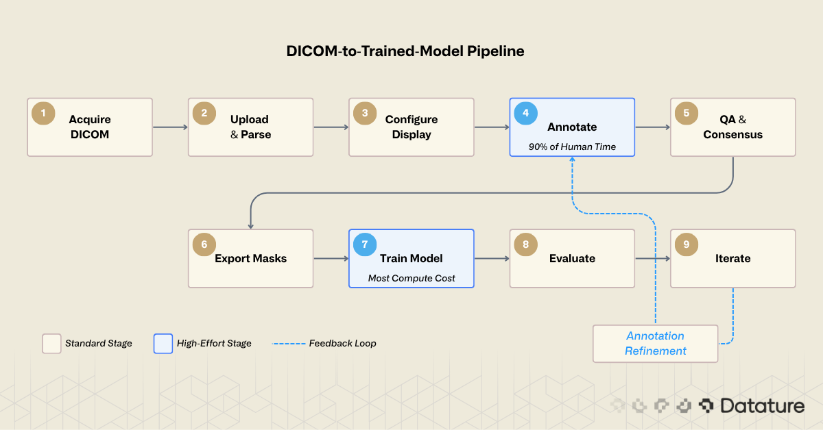
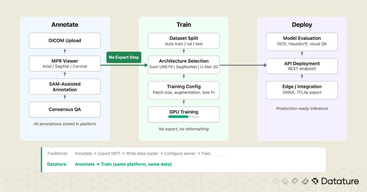
Most desktop tools cover stages 3 through 6. Most cloud platforms cover stages 2 through 6. Few cover the full chain. The gap between stage 6 (export masks) and stage 7 (train model) is where many projects lose weeks: reformatting masks, writing data loaders, configuring training infrastructure. Closing that gap is a design goal for platforms that integrate annotation and training.

Uploading and Viewing DICOM in a Cloud Platform

The first concrete step is getting your data into the annotation environment. What happens behind the upload matters. A well-built DICOM ingestion pipeline will:

• Parse the DICOM header of every file and group slices by their Series Instance UID
• Sort slices by spatial position (using the Image Position Patient tag) to reconstruct the correct slice order
• Detect and flag multi-frame DICOM files, which pack multiple slices into a single file
• Read pixel spacing and slice thickness to establish the physical voxel grid
• Apply the Rescale Slope and Rescale Intercept to convert stored values to Hounsfield units

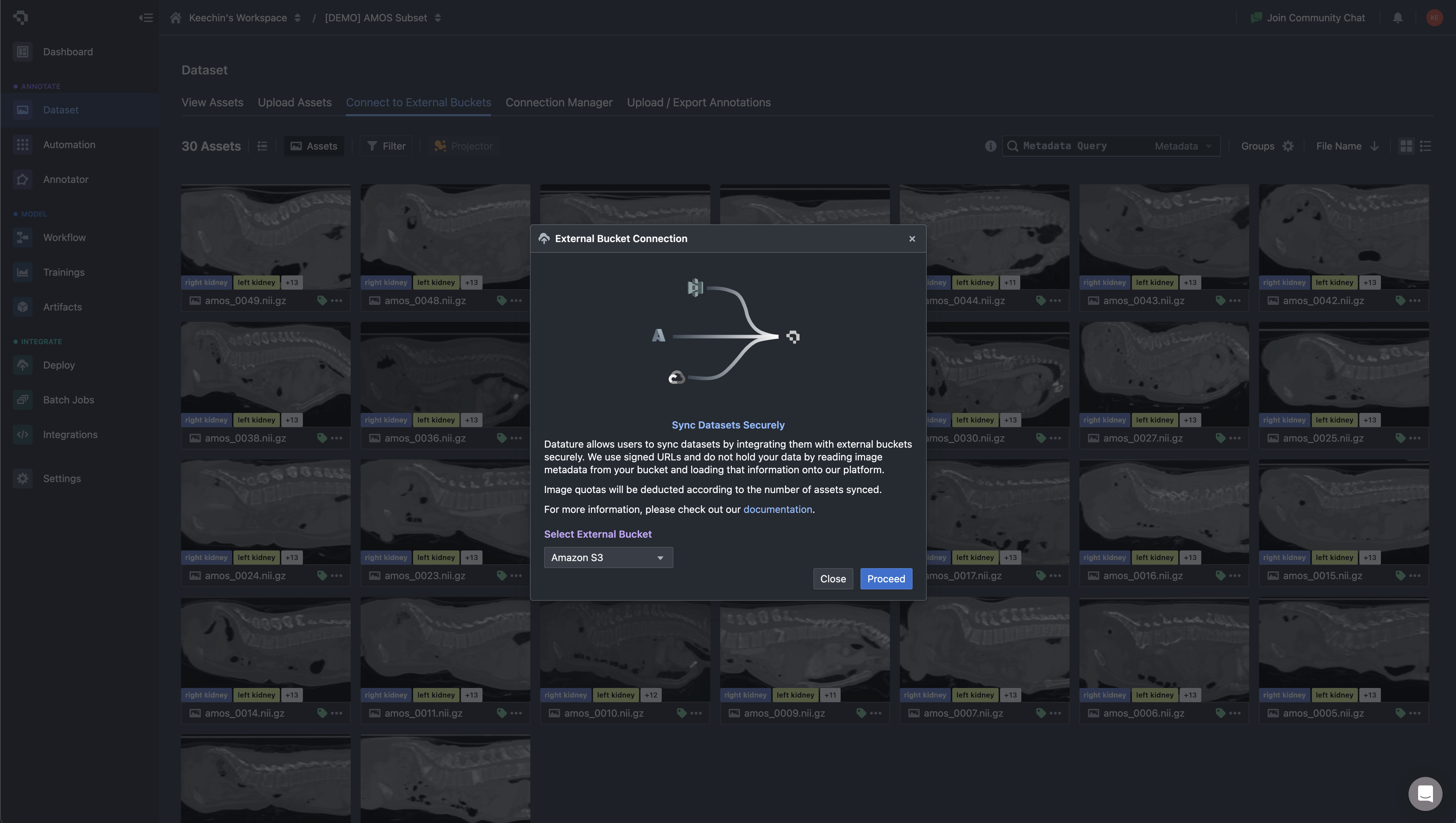
On Datature Nexus, you upload DICOM as a ZIP of .dcm files or NIfTI as .nii.gz. The platform handles series detection, slice reconstruction, and metadata extraction automatically. For teams already storing imaging data in cloud object storage, Nexus can sync directly from external buckets (Amazon S3, GCS) instead of forcing a manual upload step. Asset metadata is loaded into the platform without copying the underlying pixel data, which matters when your dataset is hundreds of gigabytes of CT volumes.

Once the volume is loaded, you work inside a three-panel multi-planar reconstruction view: axial, sagittal, and coronal planes rendered side by side, with the annotation toolbar accessible directly in the viewer. This matters for medical workflows because contour quality depends on cross-checking a structure across all three planes. A liver tumor that looks well-defined on axial may have ambiguous superior-inferior boundaries that only become clear on coronal. The annotator switches planes constantly while working, and the tool needs to keep all three views in sync.

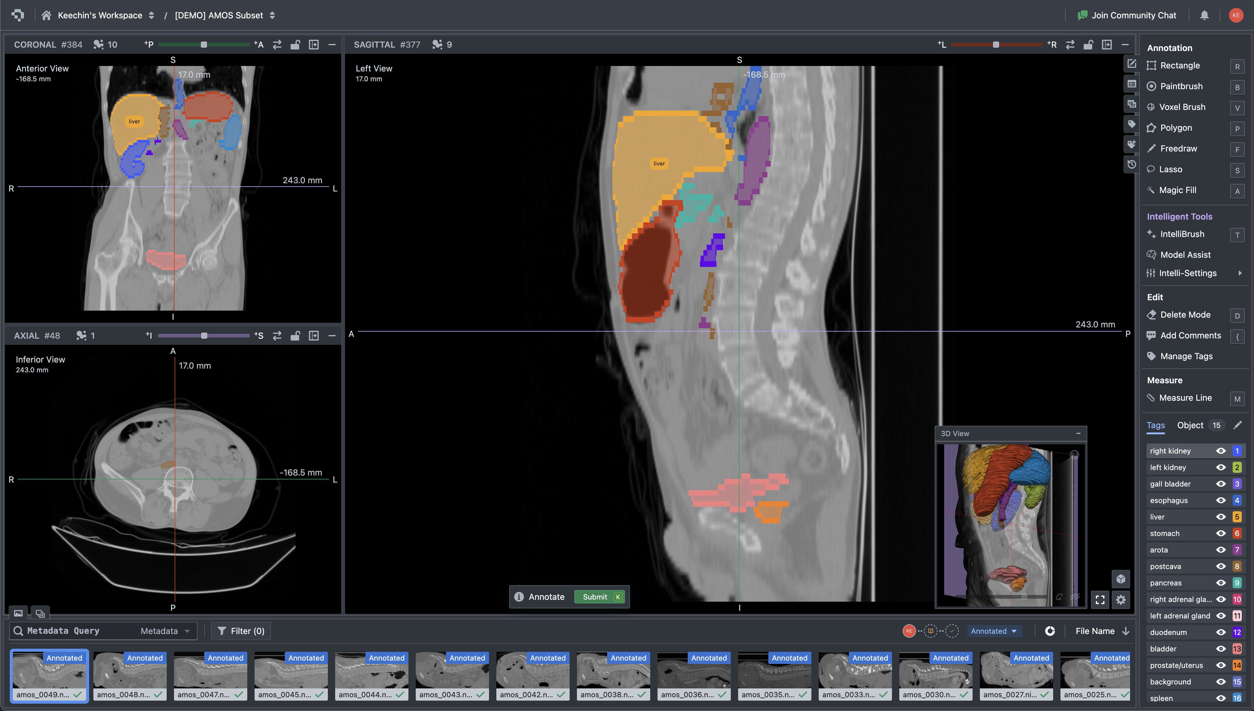
Multi-planar CT viewer with organ segmentation masks and annotation tools interface

The toolbar collapses three categories of work into one surface: manual contouring (paintbrush, polygon, lasso), volumetric operations (voxel brush, magic fill, interpolation across slices), and intelligent assistance including SAM-based interactive segmentation. The Tags panel manages the label ontology for the current dataset. For a multi-organ task like AMOS, the annotator works through 15+ structures per volume, and the tag list keeps each label distinct without forcing the user to remember color mappings.

For a step-by-step walkthrough of the upload process and supported formats, see our tutorial on uploading DICOM and NIfTI data. If you want to try the 3D annotation tools directly, the 3D medical scan annotation tutorial covers the labeling workflow.

AI-Assisted Annotation: SAM on Medical Images

Manual slice-by-slice annotation is accurate but slow. AI-assisted annotation flips the task: instead of drawing every contour from scratch, you provide minimal input (a click, a bounding box, a scribble) and the model proposes a mask that you refine. The question is which model, and how well it works on medical data specifically.

General-Purpose SAM: Strengths and Limits

Meta's Segment Anything Model (SAM) was trained on SA-1B, a dataset of 11 million natural images with over 1 billion masks. On natural photos, it generalizes well. On medical images, results are mixed. For organs with clear boundaries (liver against surrounding fat, kidneys against retroperitoneal tissue), SAM can produce usable initial masks. But it struggles with low-contrast boundaries where one soft tissue blends into another (tumor margin against brain parenchyma), small structures like lymph nodes or early-stage lesions, and 3D consistency: SAM operates on 2D slices independently, so a mask on slice 150 may not align with slice 151. For a deeper look at SAM's architecture, see our technical deep dive into SAM 3.

MedSAM and SAM-Med2D: Research Adaptations

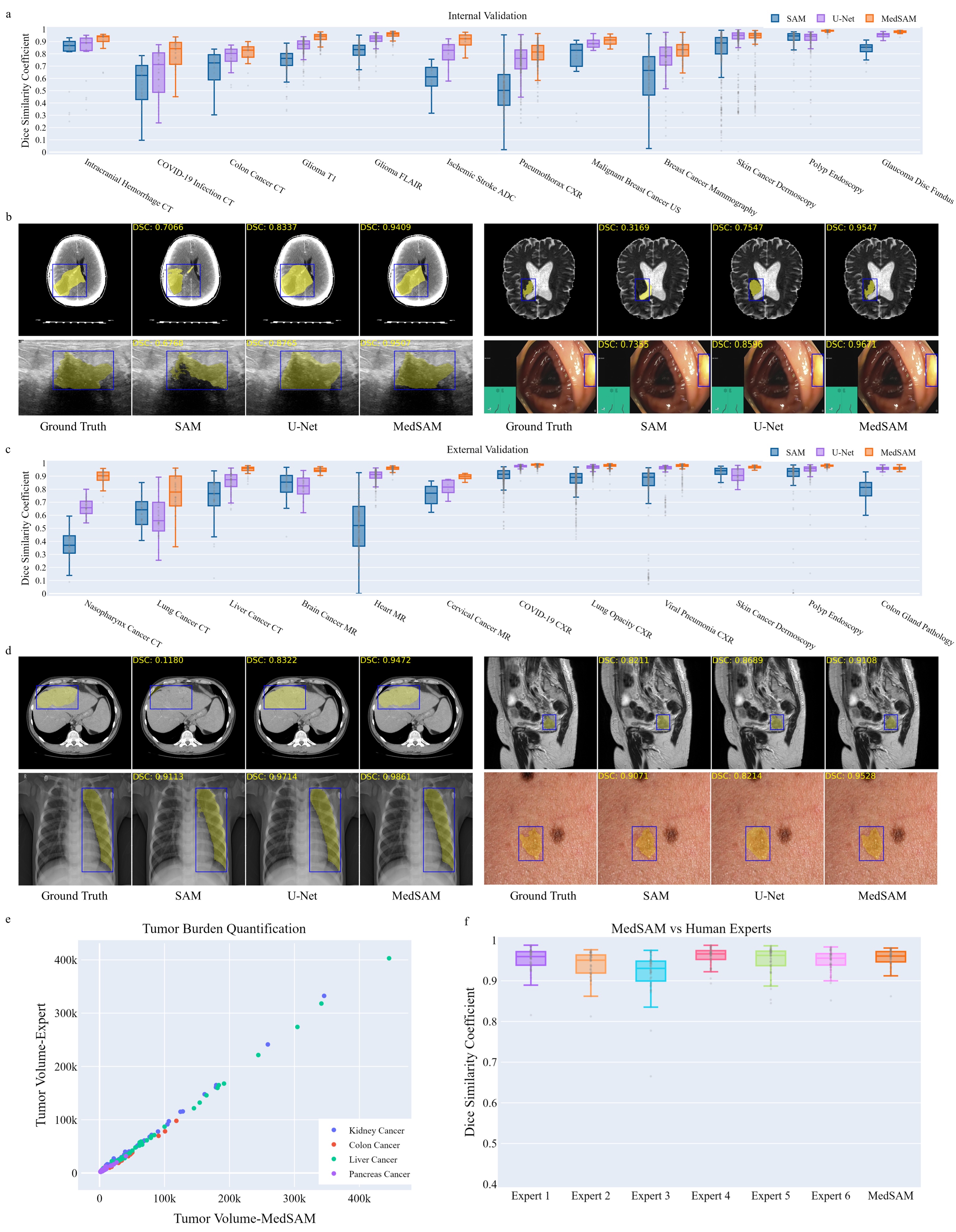
Researchers have fine-tuned SAM specifically for medical imaging. Ma et al. (2024) created MedSAM by fine-tuning on over 1.5 million medical image-mask pairs spanning 10 imaging modalities (CT, MRI, ultrasound, endoscopy, dermoscopy, X-ray, fundoscopy, OCT, pathology, microscopy).

MedSAM uses a bounding box prompt: draw a box around the target structure, and the model generates a segmentation mask. On 24 validation tasks, MedSAM outperformed vanilla SAM by 5-15 DICE points. SAM-Med2D (Cheng et al., 2023) takes a similar approach with adapter modules and prompt encoders tuned on medical data.

These medical-tuned variants are still research models. Running MedSAM requires downloading model weights, setting up a Python environment with PyTorch, and writing inference scripts. MedSAM-2 extends the approach to 3D by using SAM 2's memory attention to propagate masks across slices, though it remains similarly pre-production. The gap between general SAM and domain-tuned SAM on medical images is large enough (5-15 DICE points on the tasks tested) that these research directions matter for the field's future.

SAM in Practice: Datature's DICOM Workflow

While MedSAM and SAM-Med2D remain research-only, general-purpose SAM is available as a production tool in Datature's DICOM annotation interface. You can click on a structure or draw a bounding box directly in the MPR viewer, and SAM proposes a mask on that slice. For high-contrast structures where the organ boundary is visible against surrounding tissue (liver against fat, kidney against retroperitoneal space, aorta against lung), the initial mask is often good enough that refinement takes seconds instead of minutes per slice.

The limitation is worth stating plainly: Datature runs general SAM, not a medical-fine-tuned variant. On low-contrast boundaries (tumor margins against brain parenchyma, pancreas against surrounding bowel, early-stage lesions with minimal contrast difference), general SAM will produce rougher initial masks than MedSAM would. For those cases, you will rely more heavily on manual refinement with brush and polygon tools after SAM gives you a starting contour. The practical question is whether the time saved on high-contrast structures outweighs the extra refinement needed on difficult ones. For most multi-organ annotation projects, the answer is yes.

MONAI Label: A Different Approach

MONAI Label takes a different approach from SAM entirely. Instead of a general-purpose foundation model, it uses domain-specific models (often pre-trained on organ segmentation tasks) and improves them through an active learning loop: each correction the annotator makes gets fed back into the model. After 10 to 20 annotated volumes, the model's pre-segmentations become accurate enough to require only minor corrections. The result is often better initial masks than SAM produces on medical data, because the model has seen similar anatomy before.

The tradeoff is setup complexity. MONAI Label requires a local NVIDIA GPU, a Python environment with PyTorch and MONAI installed, and a server process connected to 3D Slicer. For teams with ML engineering support, this works well. For teams where annotators are clinicians or research assistants who need a browser-based workflow, it creates a barrier.

Multi-Annotator Workflows and Quality Control

A single annotator's segmentation is an opinion. A consensus from multiple annotators is a ground truth. This distinction matters for any project where the annotations will be used to train a model that must generalize, pass external validation, or support a regulatory submission.

Inter-annotator agreement is measured by computing the DICE coefficient between masks from different annotators for the same structure. A DICE score of 1.0 means perfect agreement. In practice, radiologists agree at roughly 0.80 to 0.90 on well-defined structures (liver, kidney) and 0.60 to 0.80 on ambiguous boundaries (tumor margins, diffuse pathology). These numbers set a ceiling: if annotators disagree at 0.75 DICE, a model that achieves 0.75 DICE is performing at human level.

A multi-annotator QA workflow typically follows this pattern:

1. Two or more annotators independently segment the same volume without seeing each other's work
2. The system computes voxel-level agreement and generates a consensus mask (majority voting, STAPLE algorithm, or weighted averaging)
3. A senior clinician reviews regions of disagreement and adjudicates the final ground truth
4. The disagreement patterns are analyzed to identify systematic issues (one annotator consistently under-segments, another includes too much surrounding tissue)

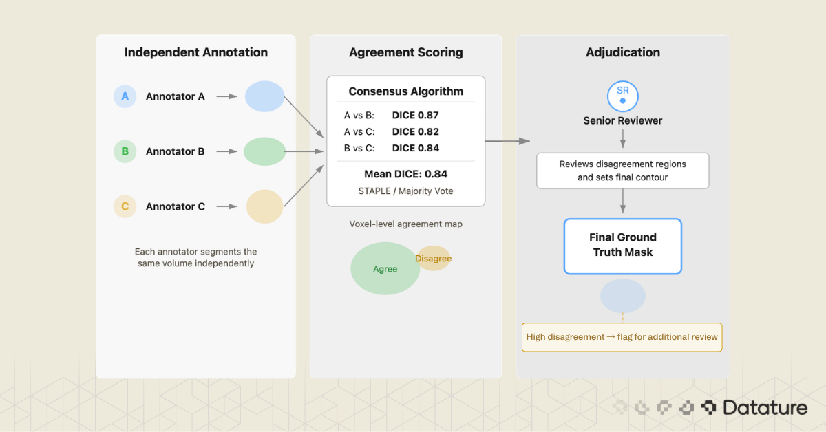
Which tools support this? 3D Slicer has no built-in multi-annotator workflow. MD.ai supports basic collaboration but lacks automated consensus scoring. Datature includes a consensus algorithm that computes inter-annotator agreement and generates merged masks with a review interface for adjudication.

From Annotations to a Trained Segmentation Model

You have annotated 200 volumes. The masks look clean. Now what?

The answer depends on what your annotation tool exports and what your training pipeline expects. This is where the "annotation-only" versus "annotation-plus-training" distinction becomes practical.

Export format matters. nnU-Net expects NIfTI masks with integer labels (0 for background, 1 for structure A, 2 for structure B). MONAI pipelines accept NIfTI or NumPy arrays. 3D Slicer uses NRRD internally. If your annotation tool exports COCO JSON (designed for 2D natural images), you will need a conversion step to produce volumetric masks, and that conversion is a common source of bugs around voxel orientation and spacing.

The gap between "exported masks" and "training run started" is wider than it looks. You need to split data by patient (not by slice, to avoid leakage), verify label mappings, confirm voxel spacing, and set up the training environment. If your annotation and training live in the same system, the mask format, label mapping, and dataset splitting can be handled automatically. This is one area where Datature's integrated pipeline removes friction: annotations flow directly into training without an export-reformat-upload cycle.

Training a 3D Segmentation Model on Annotated Data

This section gives a brief tour of the architectures you are most likely to use. For a deeper treatment of model design, training strategies, and benchmarks, read our guide to 3D models for medical image segmentation.

U-Net: The Foundation

Ronneberger et al. introduced U-Net in 2015 for biomedical image segmentation. It remains the most influential architecture in the field. The design is an encoder-decoder with skip connections: the encoder downsamples to capture context, the decoder upsamples back to full resolution, and skip connections preserve fine boundary detail. The original U-Net was 2D; extending it to 3D means replacing 2D convolutions with 3D convolutions and managing the memory increase.

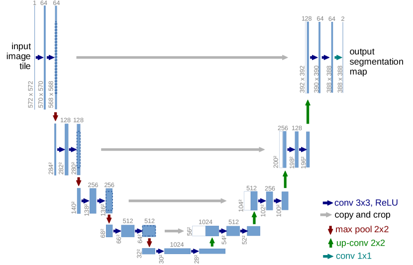
For a deeper look at FCN and U-Net architectures for segmentation, see our dedicated guide that covers the encoder-decoder design and its variants.

nnU-Net: The Self-Configuring Benchmark

nnU-Net (Isensee et al., 2021) wraps U-Net in an automated pipeline that configures preprocessing, architecture (2D, 3D full-resolution, 3D cascade), and training based on the properties of the dataset you give it. You provide labeled NIfTI files in a specific folder structure, run a command, and nnU-Net figures out the rest. It has won or placed highly in nearly every medical segmentation challenge since its release.

V-Net and SegResNet

V-Net (Milletari et al., 2016) brought two key ideas to 3D medical segmentation: residual connections inside the encoder-decoder and the DICE loss function, which handles class imbalance better than cross-entropy on small structures. SegResNet is a MONAI-native architecture that builds on similar residual encoder-decoder principles and has been used in several BraTS challenge-winning solutions.

Swin UNETR: Transformers for Volumetric Data

Swin UNETR (Hatamizadeh et al., 2022) replaces the convolutional encoder with a Swin Transformer for long-range spatial context through shifted-window self-attention. The decoder remains CNN-based with skip connections at multiple resolutions. On BraTS, Swin UNETR achieves competitive DICE scores with nnU-Net while capturing global context better, which helps with large diffuse structures like edema.

Newer contenders like MedNeXt, UNETR++, and Mamba-based architectures are appearing on challenge leaderboards, though nnU-Net remains the default benchmark that every new method must beat.

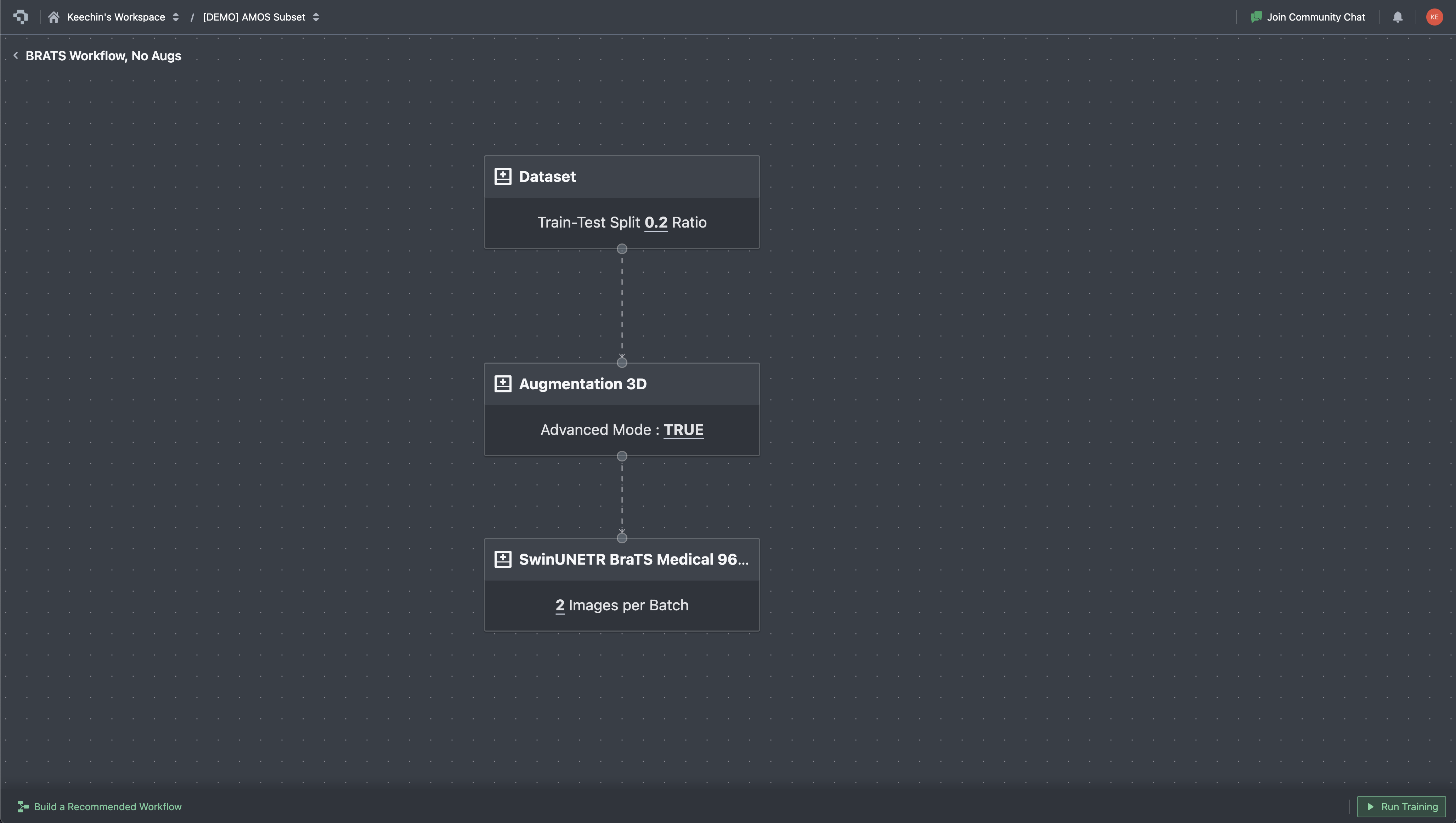
On Datature Nexus, training is configured through a visual workflow builder. Each stage is a node: dataset reference, augmentation pipeline, model architecture (Swin UNETR, SegResNet, 3D U-Net), training hyperparameters. Connect the nodes, hit Run Training, and the platform handles patch extraction, GPU provisioning, and checkpointing. This does not replace the flexibility of custom nnU-Net or MONAI scripts, but it removes the infrastructure overhead for teams that want to go from annotated data to a trained model without setting up a training server.

Once training starts, the metrics tab streams loss curves and validation scores in real time. For 3D segmentation work, the curves you watch are slightly different from a typical 2D classifier: in addition to total loss and cross-entropy, you track DICE loss (the inverse of the overlap metric you care about) and Focal loss (which keeps the model focused on rare classes when the foreground is small). MU loss appears for models with auxiliary outputs. Plotting these in real time matters because medical training runs are slow, and a plateau visible at epoch 200 saves the cost of running to epoch 1000.

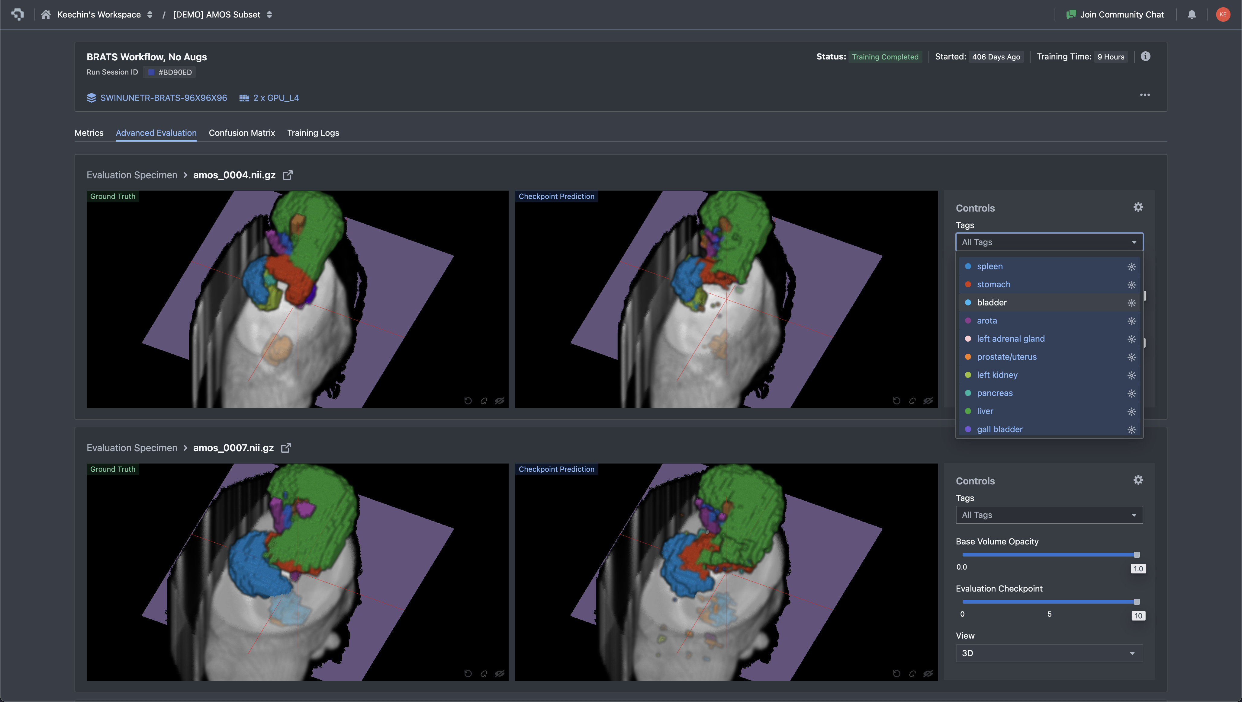
After training completes, the evaluation step is more than a DICE number on a held-out set. You need to look at the actual predictions and compare them to ground truth, slice by slice, structure by structure. A DICE score of 0.85 averaged across all classes can hide a model that nails the liver but fails on small structures like the gallbladder or adrenal gland. The Advanced Evaluation view in Nexus renders ground truth and the model's prediction side by side on the same slice, with the tag panel filtering down to a single organ at a time. Disagreements jump out visually long before they show up in a metrics table.

Where Datature Fits (and Where It Does Not)

We positioned Datature in the comparison table in Section 3 and mentioned it in several workflow sections. Here is a direct summary of where the platform is a strong fit and where it is not.

Where Datature Wins

• Cloud-native DICOM and NIfTI upload. Upload DICOM ZIPs or NIfTI files directly in the browser. The platform reconstructs volumes, renders MPR views (axial, sagittal, coronal), and supports Hounsfield unit windowing. No Python, no local install.
• Multi-planar reconstruction viewer. Three-panel MPR display with window/level controls and tissue presets. Annotators can refine contours across axial, sagittal, and coronal planes without leaving the browser.
• SAM-assisted segmentation on DICOM. Click or box-prompt SAM directly in the MPR viewer to generate initial masks on each slice. Combined with manual tools (brush, polygon, lasso) for refinement, this cuts annotation time on high-contrast structures like liver, kidneys, and major vessels. SAM operates per-slice, so manual correction is still needed for 3D consistency across the volume.
• Multi-annotator consensus. Built-in consensus algorithm computes inter-annotator DICE scores and generates merged masks with adjudication interface. Critical for teams building clinical-grade datasets.
• Annotation to training in one platform. Annotated DICOM volumes feed directly into the training pipeline (Swin UNETR, SegResNet, 3D U-Net, V-Net) without exporting, reformatting, or setting up a separate training environment.
• Deployment to API or edge. Trained models can be deployed as REST endpoints or exported as ONNX/TFLite for edge integration, closing the loop from annotation through inference.
• 3D Slicer integration. For teams that want to use both tools, Datature offers a 3D Slicer integration that connects the desktop tool with the cloud platform.

On the deployment point: a trained model exports to multiple runtimes, not just one. Nexus generates PyTorch checkpoints for further fine-tuning, ONNX for cross-framework serving, and OpenVINO for Intel-CPU edge deployment. Each export carries the model hash so you can pin a specific checkpoint to a downstream service. For teams shipping a clinical decision-support tool or research prototype, the export step is usually where vendor lock-in shows up, and being able to walk away with a portable artifact is a meaningful guarantee.

Where Datature Is Honestly Weaker

• Plugin extensibility. 3D Slicer has 500+ community plugins for specialized tasks: vessel segmentation algorithms, brain parcellation tools, cardiac analysis modules. Datature does not have a plugin ecosystem. If your workflow requires a niche algorithm that exists as a 3D Slicer extension, you need 3D Slicer.
• Community and publication track record. 3D Slicer has been used in academic research for over 20 years. Hundreds of published papers describe workflows built on it. Datature is newer in the medical imaging space, and the body of published work using it is smaller.

The honest recommendation: if you are a solo researcher with Python/3D Slicer expertise, the open-source stack (3D Slicer + MONAI Label + nnU-Net) gives you maximum control. If you are building an annotation team and want cloud collaboration, consensus QA, and annotation-to-training in one place, Datature closes gaps that desktop tools leave open. See how BrainScanology built medical AI models on Datature for a real-world example.

DICOM Annotation FAQs

What is the difference between DICOM and NIfTI for medical image segmentation?

DICOM is the clinical standard: every hospital scanner outputs DICOM, and each file carries patient metadata, scanner parameters, and pixel spacing. NIfTI is the research standard, designed for neuroimaging and later adopted across radiology research. A NIfTI file packs an entire 3D volume (or 4D time series) into one or two files, strips clinical metadata, and uses a simpler header. Most training frameworks (nnU-Net, MONAI) expect NIfTI inputs, so teams working with hospital-sourced DICOM data will convert volumes at some point in the pipeline. Cloud platforms like Datature and desktop tools like 3D Slicer accept both formats and handle the conversion internally.

What is DICOM windowing, and why does it matter for annotation?

CT pixel values are measured in Hounsfield units (HU), where air sits at -1000, water at 0, and dense bone at +1000 or higher. That range is far wider than the 256 grayscale shades a monitor can display, so the software maps a chosen slice of the HU range onto the visible spectrum using two parameters: a center (level) and a width. Common presets include lung window (center -600, width 1500), soft-tissue window (center 40, width 400), bone window (center 300, width 1500), and brain window (center 40, width 80). Choosing the wrong window makes structures invisible: a lung nodule viewed in a soft-tissue window blurs into background noise, and a liver lesion vanishes in a lung window. Datature Nexus ships standard presets for lung, soft tissue, bone, brain, and mediastinal windows, and also supports custom window/level configurations for research-specific tissue contrasts where the standard presets do not surface the features a researcher needs.

Can SAM segment medical images accurately?

General-purpose SAM (trained on 11 million natural images) works well on medical structures with clear contrast boundaries: liver against surrounding fat, kidneys, major vessels, and bony anatomy. It struggles with low-contrast boundaries where soft tissues blend together, such as tumor margins against brain parenchyma or pancreatic borders. MedSAM, a variant fine-tuned on 1.5 million medical image-mask pairs, improves performance by 5 to 15 DICE points on tested tasks but remains a research tool requiring local GPU setup. Datature offers general SAM in the DICOM annotation workflow as a production tool; it speeds up high-contrast structures while requiring more manual refinement on subtle boundaries.

What is a good DICE score for medical image segmentation?

Inter-rater agreement between trained radiologists falls in the 0.80 to 0.90 range for well-defined structures (liver, kidney, spleen) and 0.60 to 0.80 for structures with ambiguous boundaries (tumor margins, diffuse pathology). A model that matches human inter-rater DICE is performing at expert level. On public benchmarks, nnU-Net and Swin UNETR reach 0.85 to 0.92 on BraTS tumor regions and 0.80 to 0.95 across AMOS organs. Scores below 0.75 on a well-annotated dataset usually signal a problem with training data quality, class imbalance, or insufficient volume count rather than a wrong architecture choice.

How should I split DICOM data for training a 3D segmentation model?

Split by patient, not by slice. If slices from the same patient appear in both training and validation sets, the model memorizes patient-specific anatomy and validation metrics become misleadingly high. A typical split is 70/15/15 or 80/10/10 for train/validation/test. For small datasets under 50 volumes, five-fold cross-validation gives more reliable estimates than a single fixed split. Stratify by pathology type or scanner model if your dataset includes multiple sites or conditions, since a model trained only on one scanner's output may fail on another.

What is the best model architecture for 3D medical image segmentation?

nnU-Net is the default starting point. It auto-configures preprocessing, architecture variant (2D, 3D full-resolution, or 3D cascade), and training schedule based on your dataset properties, and it has won or placed highly in nearly every major medical segmentation challenge since 2021. Swin UNETR adds transformer-based long-range context that helps with large diffuse structures like edema. For teams without ML engineering resources to run nnU-Net locally, cloud platforms with built-in training (including Datature's workflow builder) offer Swin UNETR and 3D U-Net variants that can be configured without writing code.

How does cloud-based DICOM annotation compare to desktop tools like 3D Slicer?

3D Slicer offers deeper functionality for a solo researcher: 500+ community plugins, scripting via Python, and two decades of academic validation. Cloud platforms like Datature trade that plugin depth for team-scale features: browser-based access with no install, multi-annotator consensus workflows, real-time inter-rater agreement scoring, and built-in training pipelines. The deciding factors are team size and pipeline scope. A single researcher with Python experience will get more from 3D Slicer. A team of five annotators building a production dataset with QA requirements and downstream model training will spend less total time on a cloud platform.

What export formats should I look for in a medical annotation tool?

NIfTI (.nii.gz) is the most important, since nnU-Net, MONAI, and most PyTorch training pipelines expect it. NRRD matters if your workflow involves 3D Slicer for review or post-processing. COCO JSON is useful only if you plan 2D slice-level training, which is less common for volumetric tasks. On the model output side, PyTorch checkpoints let you continue fine-tuning, ONNX provides cross-framework portability, and OpenVINO covers Intel-CPU edge deployment. Datature exports trained models in all three runtime formats alongside annotation masks in NIfTI.

What if I want to train a vision-language model on medical data?

Segmentation covers image-level understanding: pixel labels, masks, organ delineation. Language tasks are a different category: summarizing radiology reports, generating findings text from scans, building chatbots over clinical images, or visual question answering on DICOM slices. For those use cases, Datature offers Datature Vi, a vision-language model platform for fine-tuning and deploying multimodal models on your own imagery and text. Vi handles the training infrastructure for VLMs the same way Nexus handles it for segmentation models, so teams working across both pixel-level and language-level tasks can stay on one platform. See the Vi fine-tuning page for specifics on supported architectures and data formats.

‍