Visual Anomaly Detection with Anomalib: A Hands-On Guide [2026]

Introduction

Manufacturing loses an estimated $10,000 per hour of unplanned downtime across industries. A large share of that cost traces back to visual defects that slip past human inspectors. Fatigue, inconsistency between shifts, and the sheer volume of parts on a modern production line make manual visual inspection unreliable at scale.

The instinct is to throw supervised deep learning at the problem: label thousands of images, train a detector, and deploy it. But here is the catch. Defects are rare. A well-run factory produces defective parts at rates below 1%. Some defect types have never been observed before. You cannot train a classifier on failure modes that do not yet exist.

Anomaly detection takes a different approach. Instead of learning what "broken" looks like, it learns what "normal" looks like. Anything that deviates from that learned distribution gets flagged. This one-class learning paradigm maps well to industrial inspection, where you have thousands of good-part images and almost no defect examples. In this guide, we will work through Anomalib, an open-source computer vision library with 23 anomaly detection algorithms, and run hands-on experiments comparing three leading approaches: PatchCore, PaDiM, and EfficientAd.

What Is Visual Anomaly Detection?

Visual anomaly detection is a computer vision technique based on one-class classification. The model sees only "normal" examples during training and learns to represent that normality as a statistical distribution, a feature space, or a reconstruction target. At inference time, any input that falls outside that learned boundary is scored as anomalous.

This differs from standard object detection and segmentation in a key way. Object detectors and segmentation models require labeled examples of every class they need to recognize, defects included. Anomaly detection needs zero defect labels. The training set contains only good samples.

That property makes anomaly detection a natural fit for defect detection in manufacturing, medical imaging (where pathological samples may be scarce), semiconductor wafer inspection, and food processing. In any domain where normal is abundant but abnormal is rare or unpredictable, the one-class approach removes the bottleneck of defect labeling. For a real-world example of anomaly detection applied to medical scans, see Datature's guide on tumor and anomaly detection in medical imaging.

Anomaly detection has trade-offs to consider. It cannot classify defect types, only flag that something is wrong. It works best when "normal" has low visual variance; products with high natural variation (wood grain, natural fabrics) may produce more false positives. And if you do have labeled defect data, a supervised defect detection model will typically outperform an unsupervised anomaly detector. The one-class approach is strongest when defect labels are scarce or when unknown defect types must be caught.

Introducing Anomalib

Anomalib is an open-source deep learning library for visual anomaly detection and automated defect detection, maintained under Intel's Open Edge Platform. Licensed under Apache 2.0, it provides a unified interface to 23 anomaly detection algorithms through both a Python API and a CLI.

The library hit version 2.2.0 in October 2025. It is built on top of PyTorch Lightning, which handles training loops, logging, and device management. Anomalib also supports OpenVINO export, making it straightforward to optimize models for Intel hardware at the edge.

What makes Anomalib practical for experimentation is its integration with standard benchmarks. It can auto-download datasets like MVTec AD and VisA, split them into train/test sets, and produce standardized metrics (Image AUROC, Pixel AUROC, F1) without manual preprocessing. For this guide, all code was tested with Anomalib 2.2.0 on Python 3.14 and PyTorch 2.10.0. We recommend Python 3.10 or higher for the best compatibility; the Anomalib CLI has known import issues on Python 3.14, though the Python API works without problems.

The MVTec AD Dataset

MVTec AD is the industry-standard benchmark for unsupervised anomaly detection. Published by MVTec Software GmbH, it contains 5,354 high-resolution images across 15 object and texture categories. Each category includes a training set of defect-free images and a test set with both normal and anomalous samples. Every anomalous test image comes with a pixel-level ground truth mask showing the exact defect region.

We will use the bottle category for our experiments. The bottle training set contains 209 normal images. The test set includes 20 normal bottles and 63 defective bottles with three defect types: broken_large, broken_small, and contamination. This mix of structural damage and surface contamination makes it a good benchmark for comparing localization quality across models.

Downloading MVTec AD

The official MVTec download URL has been unreliable since late 2025. We used the HuggingFace mirror TheoM55/mvtec_all_objects_split, which hosts the full dataset with train/test splits and ground truth masks. Here is the download script we used to fetch the bottle category and organize it into the folder structure Anomalib expects:

from datasets import load_dataset
from pathlib import Path

CATEGORY = "bottle"
OUTPUT_ROOT = Path("./datasets/MVTecAD") / CATEGORY

# Download from HuggingFace (requires: pip install datasets)
train_ds = load_dataset("TheoM55/mvtec_all_objects_split", split=f"{CATEGORY}.train")
test_ds = load_dataset("TheoM55/mvtec_all_objects_split", split=f"{CATEGORY}.test")

# Save training images (all normal/good)
train_dir = OUTPUT_ROOT / "train" / "good"
train_dir.mkdir(parents=True, exist_ok=True)
for i, sample in enumerate(train_ds):
    sample["image_path"].save(train_dir / f"{i:03d}.png")

# Save test images and masks, organized by defect type
counts = {}
for sample in test_ds:
    defect = sample["defect"]
    counts[defect] = counts.get(defect, 0) + 1
    idx = counts[defect]

    test_dir = OUTPUT_ROOT / "test" / defect
    test_dir.mkdir(parents=True, exist_ok=True)
    sample["image_path"].save(test_dir / f"{idx:03d}.png")

    if sample["label"] == 1 and sample["mask_path"] is not None:
        mask_dir = OUTPUT_ROOT / "ground_truth" / defect
        mask_dir.mkdir(parents=True, exist_ok=True)
        sample["mask_path"].convert("L").save(mask_dir / f"{idx:03d}_mask.png")

This produces the exact directory layout Anomalib expects. You can swap "bottle" for any of the 15 MVTec categories (carpet, grid, leather, tile, wood, cable, capsule, hazelnut, metal_nut, pill, screw, toothbrush, transistor, zipper) to experiment with different object types.

‍

Getting Started: Installation and Setup

Install Anomalib and its dependencies in one line:

pip install anomalib

Requirements: Python 3.10 or higher and PyTorch 2.0+. If you are using CUDA, make sure your PyTorch build matches your CUDA version.

‍

Gotcha: MVTec Download URL

The official MVTec download URL has been intermittently broken as of early 2026. Anomalib's built-in data module handles downloading automatically, but if you hit a 404 error, download the dataset manually from the MVTec AD page or use the HuggingFace mirror TheoM55/mvtec_all_objects_split. Place the extracted folder at ./datasets/MVTecAD/ and Anomalib will detect

‍

Experiment 1: PatchCore (Memory Bank Approach)

PatchCore works by extracting patch-level features from a pretrained CNN (typically a WideResNet-50), storing the most representative features in a memory bank via coreset subsampling, and scoring test images by their nearest-neighbor distance to this bank. There is no backpropagation during training. The model builds its memory bank in a single pass through the data.

from anomalib.data import MVTecAD
from anomalib.engine import Engine
from anomalib.models import Patchcore

datamodule = MVTecAD(
    root="./datasets/MVTecAD",
    category="bottle",
    train_batch_size=32,
    eval_batch_size=32,
    num_workers=4,
)

model = Patchcore(
    backbone="wide_resnet50_2",
    layers=("layer2", "layer3"),
    pre_trained=True,
    coreset_sampling_ratio=0.1,
    num_neighbors=9,
)

engine = Engine(default_root_dir="./results", max_epochs=1)
engine.fit(model=model, datamodule=datamodule)
test_results = engine.test(model=model, datamodule=datamodule)

Note: Older tutorials may use MVTec, which still works but is deprecated as of v2.2.0.

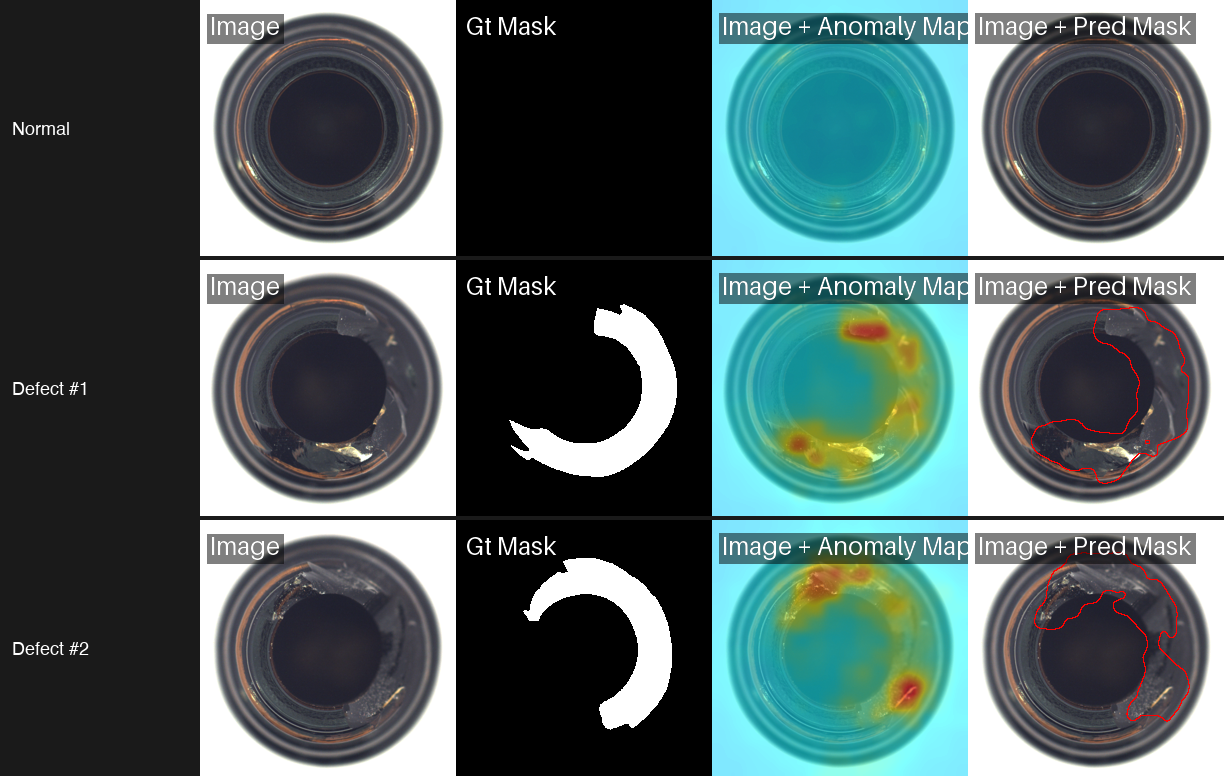
Results

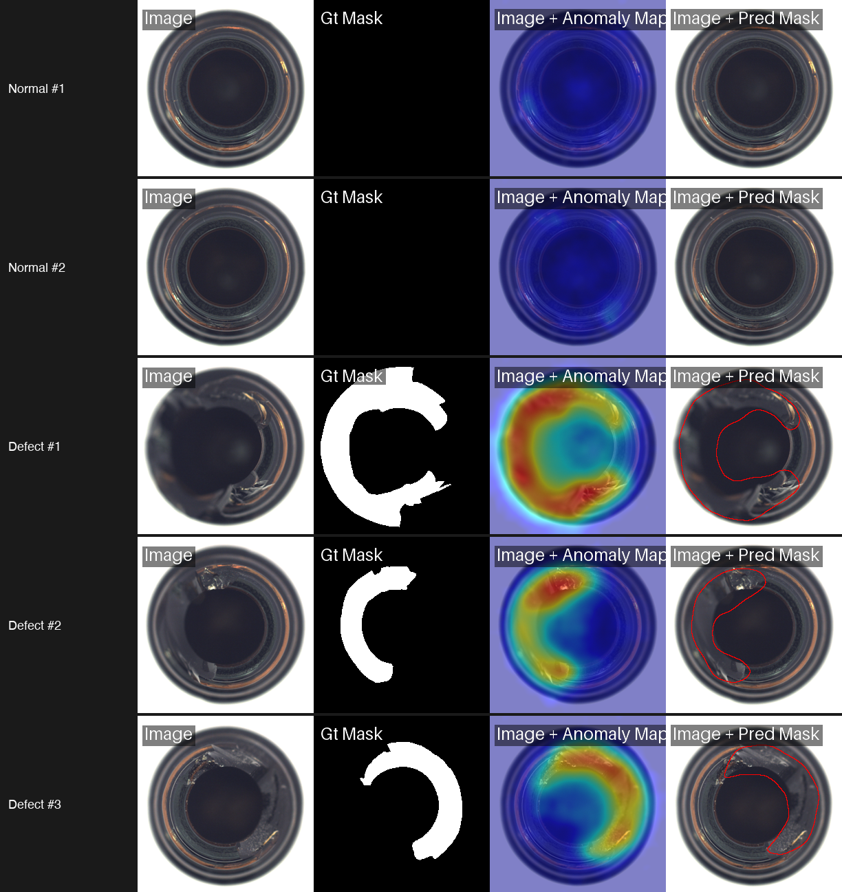
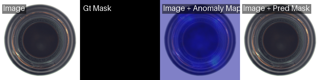
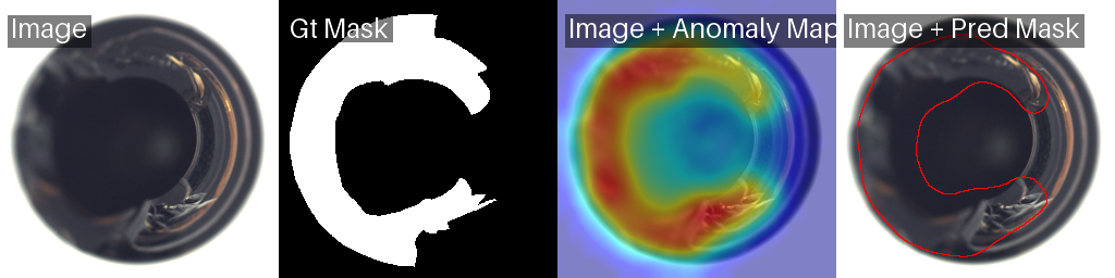
PatchCore only runs for 1 epoch because it is building a memory bank, not optimizing weights through gradient descent. The result is the best pixel-level localization of the three models we tested. The grid above shows PatchCore on normal bottles (cold heatmaps confirming no anomaly) and three defective bottles with varying break sizes. The heatmaps closely match the ground truth masks, capturing both large structural breaks and smaller damage with high precision.

Experiment 2: PaDiM (Gaussian Modeling)

PaDiM (Patch Distribution Modeling) takes a different statistical approach. It extracts patch features from a pretrained CNN at multiple layers, concatenates them into a feature vector per spatial position, and fits a multivariate Gaussian distribution to the resulting feature set. At test time, it computes the Mahalanobis distance between each patch's features and the learned Gaussian. High distances indicate anomalies.

Code

from anomalib.data import MVTecAD
from anomalib.engine import Engine
from anomalib.models import Padim

datamodule = MVTecAD(
    root="./datasets/MVTecAD",
    category="bottle",
    train_batch_size=32,
    eval_batch_size=32,
    num_workers=4,
)

model = Padim(
    backbone="resnet18",
    layers=("layer1", "layer2", "layer3"),
    pre_trained=True,
    n_features=100,
)

engine = Engine(default_root_dir="./results", max_epochs=1)
engine.fit(model=model, datamodule=datamodule)
test_results = engine.test(model=model, datamodule=datamodule)

Results

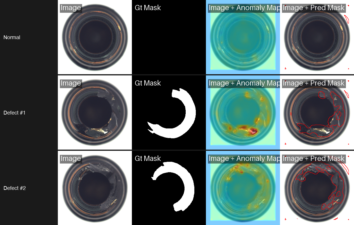
Training in 9.2 seconds compared to PatchCore's 282.8 seconds: that is a 30x speedup. And the accuracy drop is minimal, just 0.003 in pixel AUROC. PaDiM's heatmaps are slightly smoother (less granular) than PatchCore's, but they still locate defects with high precision. For rapid prototyping and resource-constrained environments, PaDiM offers the best trade-off between speed and accuracy.

Experiment 3: EfficientAd (Student-Teacher Distillation)

EfficientAd combines a lightweight autoencoder with a student-teacher knowledge distillation framework. The teacher network (a pretrained CNN) produces feature representations of normal patches. The student network learns to mimic the teacher on normal data. At inference, patches where the student's output diverges from the teacher's are flagged as anomalous.

Code

from anomalib.data import MVTecAD
from anomalib.engine import Engine
from anomalib.models import EfficientAd

datamodule = MVTecAD(
    root="./datasets/MVTecAD",
    category="bottle",
    train_batch_size=1,  # EfficientAd requires batch_size=1
    eval_batch_size=1,
    num_workers=4,
)

model = EfficientAd(
    teacher_out_channels=384,
    model_size="small",
    lr=1e-4,
    weight_decay=1e-5,
    padding=False,
    pad_maps=True,
)

engine = Engine(default_root_dir="./results", max_epochs=5)  # Paper recommends 70 epochs; we used 5 for this benchmark
engine.fit(model=model, datamodule=datamodule)
test_results = engine.test(model=model, datamodule=datamodule)

Results

*Trained for 5 of the recommended 70 epochs. Full training would improve pixel AUROC.

EfficientAd produces the most focused heatmaps of the three. Instead of broad warm regions, it highlights tight clusters around the exact defect location. The pixel AUROC is lower than PatchCore and PaDiM on this specific benchmark, but EfficientAd was designed for inference speed on edge devices. Its lightweight architecture makes it the right choice when you need real-time scoring on constrained hardware.

Model Comparison

All three models achieved perfect image-level AUROC (1.000) on the MVTec AD bottle category. The differences show up in pixel-level localization and training time.

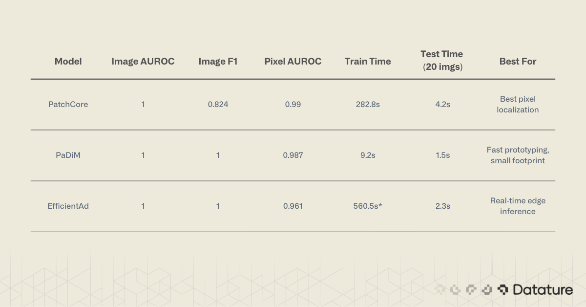
PaDiM and EfficientAd both achieved perfect Image F1 (1.000), while PatchCore scored 0.824. This means PaDiM made zero false-positive or false-negative errors at the image level.

Comparison of PatchCore, PaDiM, and EfficientAd showing anomaly heatmaps and predicted defect masks on bottle image - with the same dataset good and bad split.

When to Use Which Model

PatchCore is the right starting point when localization accuracy matters most and you have enough memory to store the coreset. For defect detection on manufacturing inspection lines, where defect location drives repair decisions, PatchCore's precise heatmaps are the best option.

PaDiM is the best choice for rapid iteration. If you are prototyping across dozens of product categories or running experiments on a laptop, the 9-second training time removes friction. The accuracy penalty is negligible for most practical applications.

EfficientAd targets deployment scenarios. Its student-teacher architecture produces a compact model that runs at camera-rate speeds on edge hardware. If your production line needs sub-100ms inference, start here.

For readers exploring beyond these three models, Dinomaly (published at CVPR 2025) holds the current state-of-the-art on MVTec AD with 99.6% image AUROC across all 15 categories. It is available in Anomalib v2.2.0 as anomalib.models.Dinomaly and uses a DINOv2 vision transformer backbone.

For a deeper look at how metrics like AUROC, precision, and recall relate to model evaluation, see this guide on evaluating computer vision models with confusion matrices.

Running Inference on Single Images

After training, you often need to score individual images rather than run a full test set. Anomalib's Engine provides a predict method for this. Here we load a PaDiM checkpoint and run inference on a single image.

from pathlib import Path
from anomalib.engine import Engine
from anomalib.models import Padim

# Load the trained model from a checkpoint
checkpoint = Path("./results/Padim/mvtec_bottle/v0/weights/lightning/model.ckpt")
model = Padim.load_from_checkpoint(checkpoint)
model.eval()

# Run inference on a single image
engine = Engine(accelerator="auto")
predictions = engine.predict(
    model=model,
    data_path="path/to/your/image.png",
)

# Extract results
batch = predictions[0]
score = batch.pred_score[0].item()       # anomaly score (0-1)
label = batch.pred_label[0].item()       # True = anomalous
anomaly_map = batch.anomaly_map[0]       # pixel-level heatmap (H, W)
pred_mask = batch.pred_mask[0]           # binary segmentation mask (H, W)

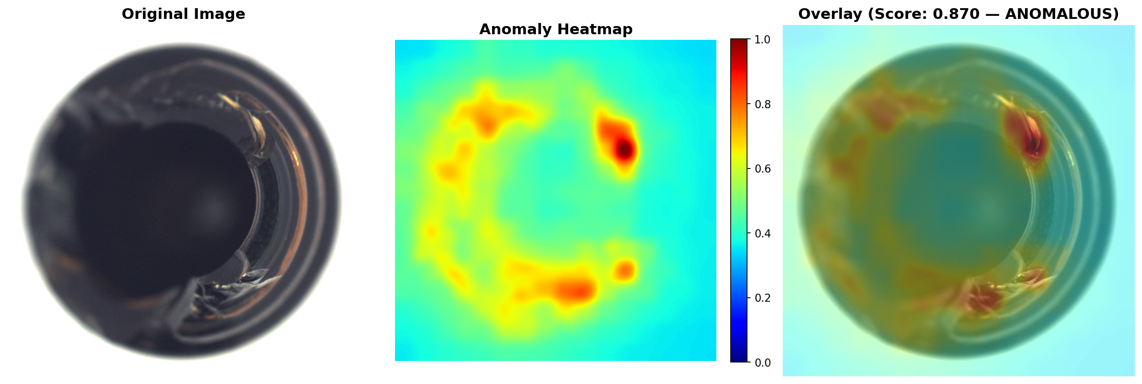
print(f"Anomaly score: {score:.4f}")
print(f"Prediction: {'ANOMALOUS' if label else 'NORMAL'}")

In our tests, a defective bottle with visible contamination scored 0.87 (labeled ANOMALOUS), while a clean bottle scored 0.25 (labeled NORMAL). The anomaly_map tensor contains the full pixel-level heatmap, which you can overlay on the original image for visual inspection. The pred_mask gives you a binary segmentation of the anomalous region. This could be helpful in cases where you want to either quantify the severeity of the anomaly in your images, beyond just obtaining the outline.

Training on Your Own Dataset

Anomalib supports custom datasets through the Folder data module. The key requirement is directory structure: your training set must contain only normal (good) images. The test set can include both normal and anomalous samples.

How Labeling Works: Folder-Based, No Annotations Needed

This is one of the most practical things about anomaly detection. There are no bounding boxes to draw, no polygons to trace, no label files to manage. Your "labeling" is sorting images into folders.

Put good parts in train/good/. Put good test samples in test/good/. Put defective test samples in test/defect/. That's it. The folder name is the label. The model learns from the train/good/ folder what "normal" looks like, and at test time, anything placed in test/defect/ is compared against that learned distribution.

If you want pixel-level evaluation metrics (not just image-level scores), you can optionally add binary segmentation masks in a ground_truth/ folder. Each mask is a simple black-and-white PNG where white pixels mark the defect region. These masks are only used for scoring, not for training. The model never sees them during the learning phase.

For most teams starting out, skip the masks entirely. Collect 50-200 images of your product in good condition, drop them into train/good/, and run PaDiM. You will have a working anomaly detector in under a minute.

Folder Structure

my_dataset/
  train/
    good/           # Only normal images here (50+ recommended)
  test/
    good/           # Normal test images
    defect/         # Anomalous test images
  ground_truth/
    defect/         # Optional: binary masks for pixel-level evaluation

Code

from anomalib.data import Folder
from anomalib.engine import Engine
from anomalib.models import Padim

datamodule = Folder(
    name="my_dataset",
    root="./my_dataset",
    normal_dir="train/good",
    abnormal_dir="test/defect",
    normal_test_dir="test/good",
    mask_dir="ground_truth/defect",  # optional
    train_batch_size=32,
    eval_batch_size=32,
    num_workers=4,
)

model = Padim(backbone="resnet18", pre_trained=True)
engine = Engine(default_root_dir="./results", max_epochs=1)

engine.fit(model=model, datamodule=datamodule)
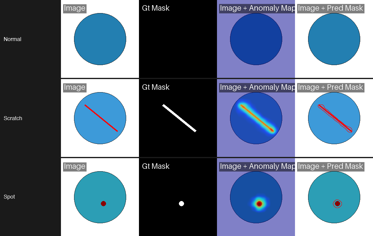
engine.test(model=model, datamodule=datamodule)

In our test with 50 training images of circles on white backgrounds, PaDiM learned the normal distribution in 3 seconds and detected scratches and spots on test circles with near-perfect accuracy. The critical point: your training set must contain only defect-free examples. Any contamination in the training data teaches the model to treat defects as normal.

For tips on preparing and inspecting your datasets before training, see Datature's guide on visually inspecting datasets and annotations for model training.

CLI Quick Reference

Anomalib also supports a command-line interface for users who prefer shell-based workflows:

# Train PaDiM on MVTec AD bottles
anomalib train --model Padim --data anomalib.data.MVTec \
  --data.category bottle --data.root ./datasets/MVTecAD

# Train PatchCore on a custom folder dataset
anomalib train --model Patchcore --data anomalib.data.Folder \
  --data.root ./my_dataset --data.normal_dir good \
  --data.abnormal_dir defective

# Run prediction on new images
anomalib predict --model Patchcore \
  --ckpt_path ./results/Patchcore/latest/weights/lightning/model.ckpt \
  --data.path ./new_images/

# Export to OpenVINO format for edge deployment
anomalib export --model Patchcore \
  --ckpt_path ./results/Patchcore/latest/weights/lightning/model.ckpt \
  --export_type openvino

The CLI mirrors the Python API. Any model or dataset configuration available in code can be specified as command-line arguments.

Python 3.14 Compatibility

The Anomalib CLI has known compatibility issues on Python 3.14. If you encounter import errors, use the Python API instead or switch to Python 3.10-3.12.

Tips and Gotchas

Working through these experiments, we hit several issues that are not well-documented. Here is what to watch for:

MVTec Download URL

As of early 2026, the official MVTec download endpoint fails intermittently with 404 errors. Download manually from the MVTec website or use the HuggingFace mirror TheoM55/mvtec_all_objects_split.

‍

Class naming. Anomalib uses Patchcore (not PatchCore), Padim (not PaDiM), and EfficientAd. The inconsistent casing trips up imports. Check anomalib.models if autocomplete gives you the wrong name.

EfficientAd batch size. EfficientAd requires batch_size=1 for both training and evaluation. Setting it higher throws a shape mismatch error during the student-teacher comparison step.

macOS workers. On macOS, set num_workers=0 to avoid multiprocessing issues with PyTorch's DataLoader. The performance hit is minor for small datasets like MVTec AD.

Prediction output format. The engine.predict() method returns ImageBatch objects, not dictionaries. Access scores with .pred_score, labels with .pred_label, and heatmaps with .anomaly_map. This changed from earlier Anomalib versions that used plain dicts.

Image size matters. Anomalib resizes inputs to 256x256 by default. If your images contain small defects that get lost at this resolution, increase the image_size parameter in the data module. This increases training time and memory use but improves localization on fine-grained defects.

For more context on interpreting the training metrics these models produce, see this walkthrough on understanding training graphs and model performance.

From Experiments to Production

Anomalib is a powerful computer vision tool for prototyping and benchmarking anomaly detection models. But moving from a Jupyter notebook to a production inspection line introduces new challenges: managing labeled datasets across teams, retraining as product lines change, deploying models to edge devices on the factory floor, and monitoring model drift over time.

Anomaly Detection on Datature Nexus

Datature Nexus will be supporting anomaly detection models under classification projects. The workflow maps directly to what we covered in this guide. Upload your normal images, tag them with a "good" class label, and train a classification model that learns the boundary between normal and anomalous. Nexus handles the data versioning, training infrastructure, and deployment pipeline so your team can focus on collecting good reference images rather than managing ML tooling.

For teams that want to go beyond binary good/bad classification, Nexus also supports object detection and segmentation workflows. You can start with anomaly detection to catch defects, then train a detection model to localize and categorize specific defect types as your labeled dataset grows. Companies like Ingroth and Trendspek use Datature to build and maintain their inspection pipelines at scale.

Image augmentation is another technique that can help stretch small defect datasets further, and Datature's guide on performing image augmentation for machine learning covers the practical details.

Conclusion

Anomaly detection turns the usual supervised learning requirement on its head. Instead of collecting and labeling hundreds of defect examples, you train on what you already have: images of good parts. The three models we tested each fill a different niche. PaDiM trains in under 10 seconds and delivers strong accuracy, making it the best entry point for quick experiments. PatchCore pushes pixel-level localization to near-perfect scores when accuracy is the priority. EfficientAd trades some localization precision for a model architecture designed to run at production speeds on edge devices.

Anomalib wraps all of these approaches (and 20+ more) into a single library with consistent APIs, auto-downloading datasets, and OpenVINO export. The defect detection workflow applies across industries, from semiconductor wafer inspection to food quality screening to pharmaceutical packaging: collect normal images, pick a model, train, and deploy. No deep computer vision expertise is required to get started. Start with PaDiM to prove the concept. Graduate to PatchCore when you need the best localization. Move to EfficientAd when inference speed becomes the bottleneck.