Image Augmentation for Machine Learning: Techniques, Examples & Code

A trained model is only as good as the data behind it. Feed it 500 nearly identical images of a stop sign, and it will recognize stop signs on sunny days from one angle. Show it a stop sign at dusk, rotated 15 degrees, partially occluded by a tree branch? It fails.

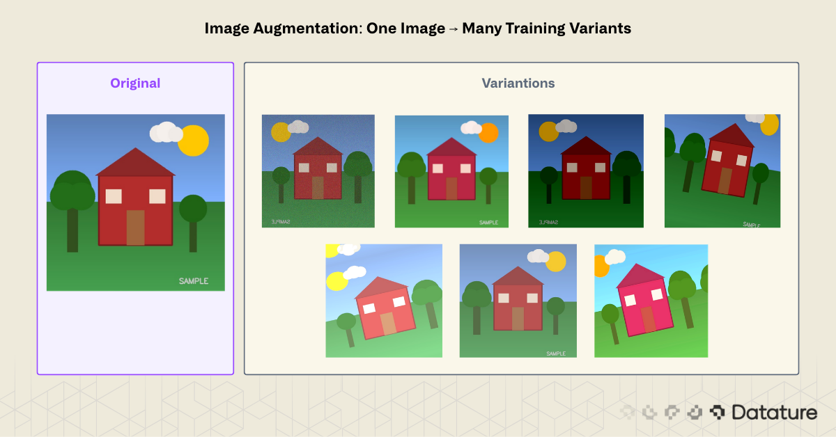
This is the core problem image augmentation solves. By applying controlled transformations to existing training images, you create synthetic variations that teach models to generalize. A single photograph of a stop sign becomes dozens: rotated, brightened, cropped, flipped, color-shifted. The model learns to recognize the concept of a stop sign rather than memorizing pixel patterns from a fixed viewpoint.

Image augmentation is one of the most cost-effective ways to improve model accuracy. Collecting and labeling new images costs time and money. Augmenting existing data costs compute cycles and nothing else. For teams working with small datasets (under 10,000 images) or in domains where data collection is restricted, such as medical imaging or rare defect detection, augmentation often makes the difference between a usable model and one that overfits on training data.

This guide covers the theory behind augmentation, walks through 12+ techniques grouped by category, compares popular Python libraries (Keras ImageDataGenerator vs. Albumentations), and shows how to apply augmentation in a no-code workflow using Datature's platform.

What Is Image Augmentation?

Image augmentation is a data preprocessing technique that generates new training samples by applying geometric, photometric, or erasing transformations to existing images. The original labels carry over to the augmented copies. A bounding box around a dog stays valid after a horizontal flip; a segmentation mask rotates with the image.

The goal is to increase the effective size and diversity of a training dataset without collecting new raw data. Augmentation acts as a regularizer: by showing the model slightly different versions of the same object, it reduces overfitting and improves performance on unseen data.

Two key properties separate good augmentation from bad:

1. Label-preserving: The transformation must not change what the image represents. Flipping a photo of a cat horizontally still shows a cat. But flipping the digit "6" vertically turns it into a "9," which changes the label. Augmentation strategies must account for the task.
2. Realistic: Transformations should mimic variations the model will encounter at inference time. An outdoor surveillance model benefits from brightness jitter and rain simulation. A satellite imagery model benefits from rotation (since orientation is arbitrary) but not vertical flipping (buildings don't appear upside-down).

How Augmentation Fits in the ML Pipeline

Augmentation typically happens at one of two stages:

• Offline (pre-training): Generate augmented copies ahead of time and save them to disk. This increases storage requirements but makes training straightforward. Useful when augmentations are expensive to compute.
• Online (during training): Apply random transformations on-the-fly as each batch loads. Each epoch sees different augmented versions of the same image. This approach is more memory-efficient and produces greater variety since the model never sees the exact same augmentation twice.

Most modern training pipelines use online augmentation. Libraries like Albumentations and TorchVision Transforms make this straightforward.

When Augmentation Helps Most

Augmentation provides the largest gains in three scenarios:

• Small datasets (under 5,000 images): Models overfit quickly without enough variation. Augmentation can double or triple effective dataset size.
• Class imbalance: If one class has 10x fewer samples than another, targeted augmentation on the minority class helps balance the distribution. For more on this, see Solving Class Imbalance: Upsampling in Machine Learning Projects.
• Domain-specific variation: When the deployment environment introduces variation not present in training data (lighting changes, camera angles, weather conditions), augmentation can simulate these conditions.

Augmentation is not a substitute for collecting more data. A model trained on 100 augmented images of a single dog breed will not generalize to other breeds. But when paired with a well-curated dataset, augmentation consistently closes the gap between training and real-world performance.

Types of Image Augmentation

Augmentation techniques fall into four categories: geometric, photometric, erasing, and mixing. Each category targets a different source of real-world variation.

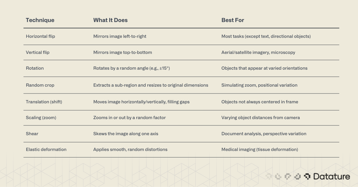
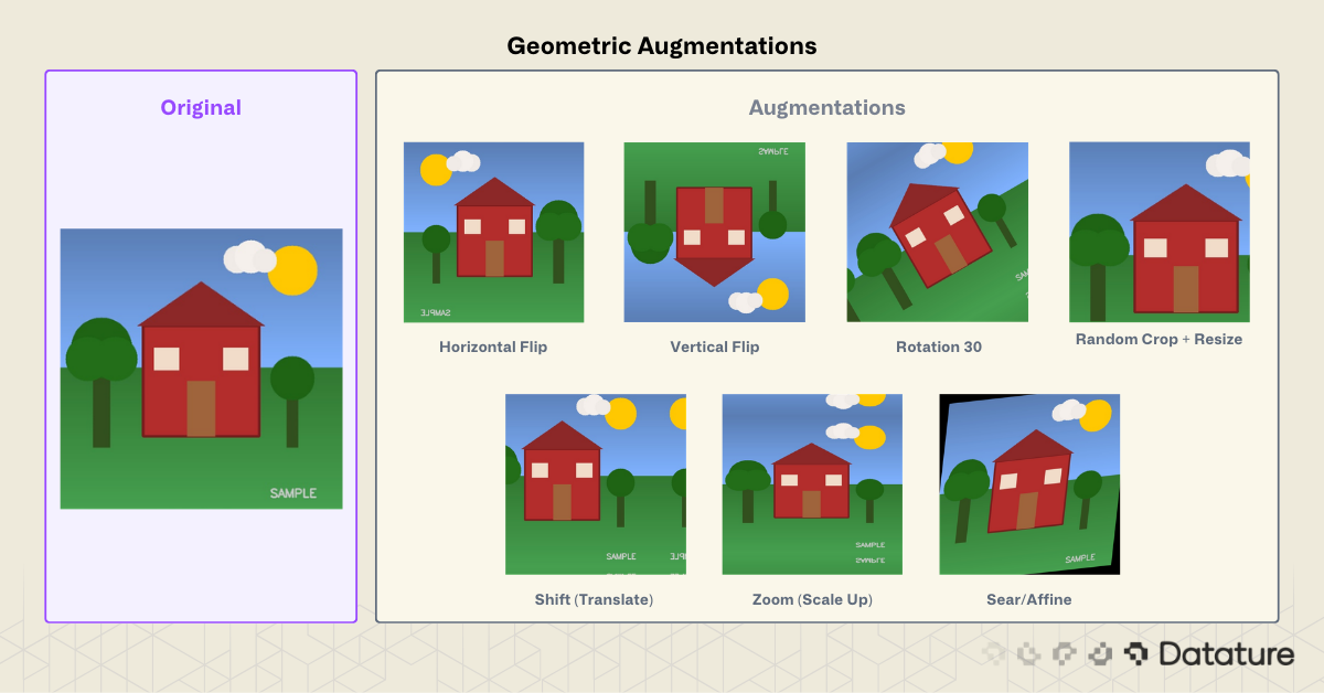
Geometric Augmentations

Geometric transforms change the spatial arrangement of pixels. They simulate variations in camera position, angle, and distance.

Watch out for annotation alignment. When augmenting detection or segmentation datasets, bounding boxes and masks must transform along with the image. Albumentations handles this automatically. Manual Keras pipelines require extra code.

Photometric (Color Space) Augmentations

Photometric transforms change pixel intensity, color, or contrast without moving them. They simulate lighting changes, camera sensor variation, and weather effects.

A note on color augmentation strength. Small jitter values (±10-20% brightness) help generalization. Extreme values (±50%) can create unrealistic images that hurt performance. Start conservative and increase only if validation metrics improve.

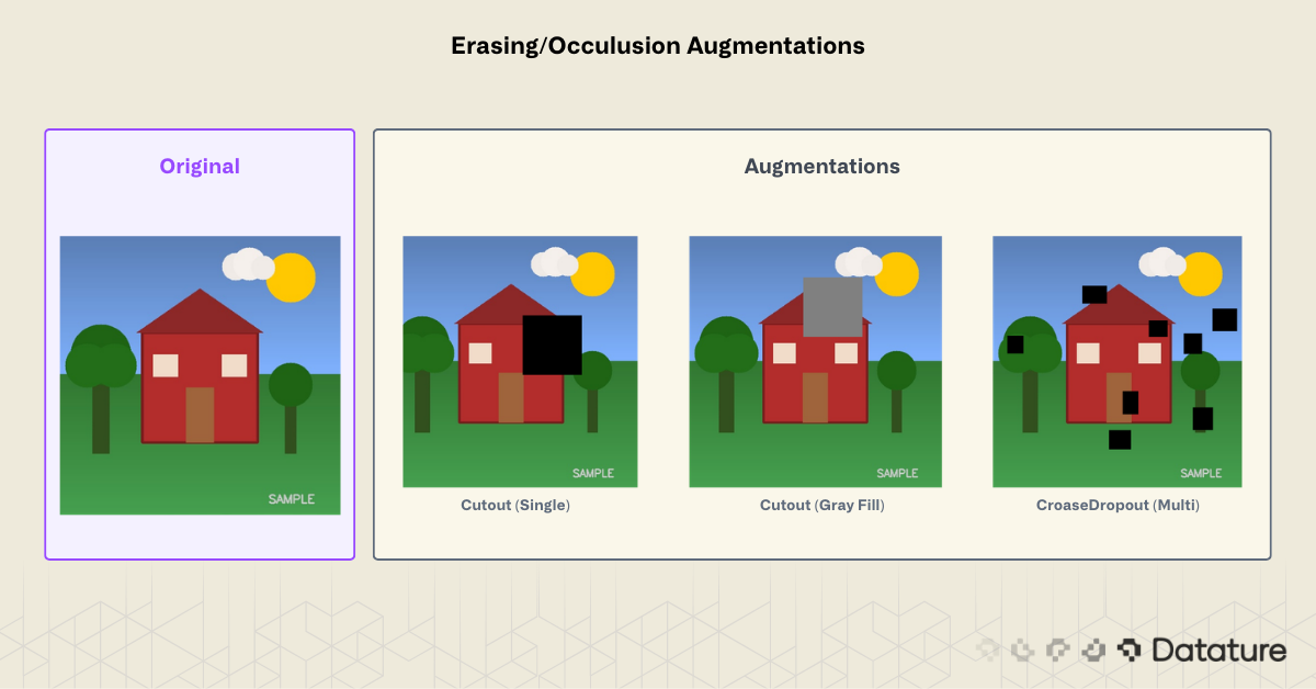
Erasing and Occlusion Augmentations

These techniques randomly remove or mask parts of the image. They force the model to rely on multiple features rather than a single discriminative region.

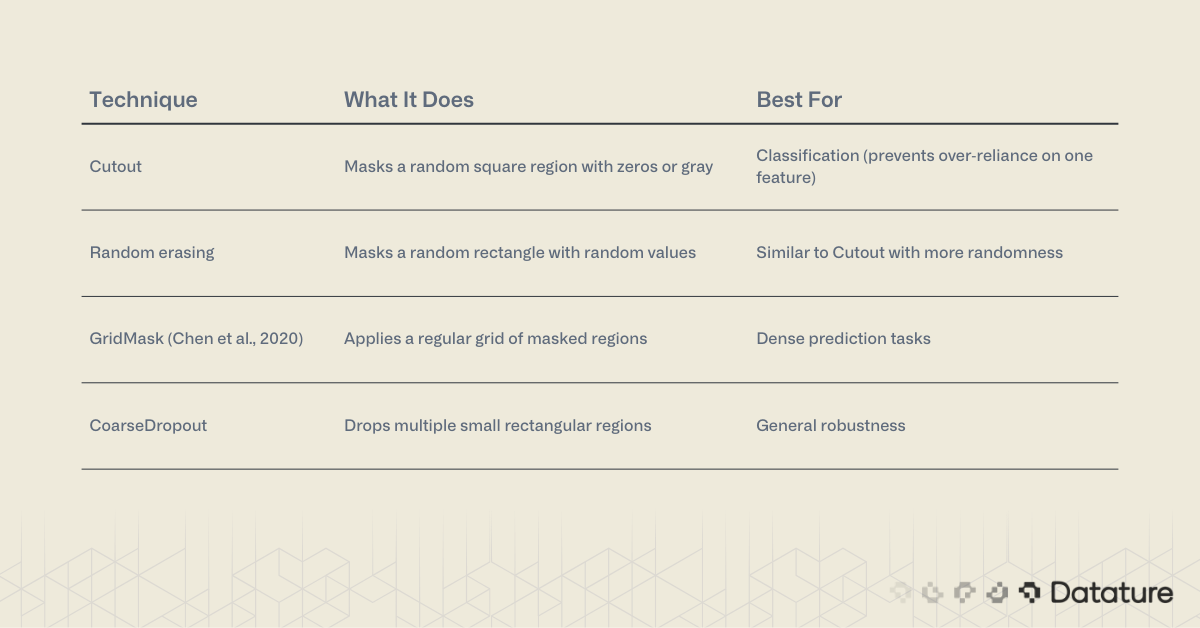
Cutout was introduced by DeVries and Taylor (2017). The idea: if a model can classify an image correctly even with part of it missing, it has learned redundant, distributed features rather than relying on a single discriminative patch. The original paper used 16x16 patches on CIFAR-10 (50% of the 32x32 image). In practice, cutout sizes of 20-30% of the image dimension are a common starting point for larger images, though the optimal size depends on object scale and dataset.

Mixing Augmentations

Mixing augmentations combine two or more images to create new training samples. They produce strong regularization but change the label: the resulting image gets a weighted combination of the original labels.

How Mixup works mathematically. Given two training samples (x_i, y_i) and (x_j, y_j), Mixup creates a new sample:

x_new = λ * x_i + (1 - λ) * x_j
y_new = λ * y_i + (1 - λ) * y_j

where λ is sampled from a Beta distribution: λ ~ Beta(α, α). The hyperparameter α controls blend strength (α=0.2 is a common default). Because the label y_new is a soft mixture rather than a hard one-hot vector, the loss function must handle soft targets (standard cross-entropy with label smoothing or KL divergence).

CutMix extends this by cutting a rectangular patch from one image and pasting it onto another. The label weight equals the area ratio of the pasted patch. This forces the model to attend to all spatial regions, combining the benefits of Cutout (occlusion robustness) with Mixup (label smoothing).

Mosaic augmentation deserves special attention for object detection. Used in YOLOv4 and later versions, it tiles four training images into a single composite, forcing the model to detect objects at different scales and in varied contexts. Mosaic contributes to YOLO's multi-scale detection capability, alongside the FPN/PAN feature pyramid neck that fuses features across resolutions.

Advanced and Domain-Specific Techniques

Some tasks benefit from specialized augmentations:

• Style transfer augmentation: Apply neural style transfer to vary texture while preserving structure. Used in domain adaptation (e.g., training on synthetic data, deploying on real).
• Weather simulation: Add synthetic rain, fog, or snow to outdoor scenes. Libraries like imgaug and Albumentations offer these.
• Photometric distortion sequences: Chain multiple color transforms in random order. The SSD paper (Liu et al., 2016) popularized this approach.
• Test-time augmentation (TTA): Apply augmentations at inference, then average predictions across augmented versions. Typical TTA pipelines use horizontal flip + 2-3 scale factors, averaging the softmax outputs. This costs 3-5x inference time but reliably boosts accuracy by 1-3% on benchmarks. Use it when accuracy matters more than latency (e.g., medical diagnosis, competition submissions).

Learned Augmentation Policies: AutoAugment, RandAugment, TrivialAugment

Manually choosing augmentation techniques and tuning their parameters is time-consuming. A family of methods automates this process:

• AutoAugment (Cubuk et al., 2019) uses reinforcement learning to search for the best augmentation policy on a given dataset. It found that different datasets prefer different augmentation combinations. The downside: the search itself requires thousands of GPU hours.
• RandAugment (Cubuk et al., 2020) simplified AutoAugment to just two hyperparameters: N (number of transforms to apply) and M (magnitude of each transform). Despite the simplicity, RandAugment matches or beats AutoAugment on most benchmarks. This is the practical default for many training recipes.
• TrivialAugment (Mueller & Hutter, 2021) went further: zero hyperparameters. It randomly selects one augmentation per image and samples its magnitude uniformly. It matches RandAugment with no tuning at all.

These methods are available in TorchVision (torchvision.transforms.v2.RandAugment, TrivialAugmentWide) and Albumentations. If you're training a classification model and don't want to hand-pick augmentations, start with RandAugment(N=2, M=9) or TrivialAugment.

# TorchVision RandAugment example
import torch
from torchvision.transforms import v2

transform = v2.Compose([
    v2.RandAugment(num_ops=2, magnitude=9),
    v2.RandomHorizontalFlip(p=0.5),
    v2.ToImage(),
    v2.ToDtype(torch.float32, scale=True),
    v2.Normalize(mean=[0.485, 0.456, 0.406],
                 std=[0.229, 0.224, 0.225]),
])

Comparing Augmentation Libraries

Three libraries cover most Python augmentation needs: Albumentations, TorchVision v2 Transforms, and the legacy Keras ImageDataGenerator.

Keras ImageDataGenerator (Legacy)

Deprecation note:

‍ImageDataGenerator was deprecated in TensorFlow 2.9 (2022). For new TensorFlow projects, use tf.keras.layers preprocessing layers or tf.data pipelines with tf.image ops. The code below is included because many existing tutorials and codebases still reference this API.

‍

Keras ships with ImageDataGenerator as part of tf.keras.preprocessing.image. It was historically the simplest way to add augmentation to a TensorFlow pipeline.

from tensorflow.keras.preprocessing.image import ImageDataGenerator

datagen = ImageDataGenerator(
    rotation_range=20,
    width_shift_range=0.15,
    height_shift_range=0.15,
    horizontal_flip=True,
    vertical_flip=False,
    brightness_range=[0.8, 1.2],
    zoom_range=0.15,
    fill_mode="nearest"
)

# Generate augmented batches from a directory
train_generator = datagen.flow_from_directory(
    "data/train",
    target_size=(224, 224),
    batch_size=32,
    class_mode="categorical"
)

Strengths: Zero extra dependencies (comes with TensorFlow), simple API, integrates directly with model.fit().

Limitations: Only supports geometric and basic color transforms. No Cutout, no Mosaic, no bounding box or mask transforms. Slower than Albumentations. Officially deprecated in favor of tf.keras.layers preprocessing layers.

The code below generates an 8×8 grid of augmented images to visually verify that transforms look reasonable:

import matplotlib.pyplot as plt
import numpy as np
from tensorflow.keras.preprocessing.image import load_img, img_to_array

img = load_img("container.jpg", target_size=(256, 256))
img_array = img_to_array(img)
img_array = np.expand_dims(img_array, axis=0)

fig, axes = plt.subplots(8, 8, figsize=(16, 16))
aug_generator = datagen.flow(img_array, batch_size=1)
for ax in axes.flat:
    ax.imshow(next(aug_generator)[0].astype("uint8"))
    ax.axis("off")
plt.tight_layout()
plt.savefig("augmentation_grid.png", dpi=150)
plt.show()

Albumentations

Albumentations is the go-to library for production augmentation pipelines. It supports 70+ transforms, handles bounding boxes, keypoints, and segmentation masks natively, and historically benchmarks 2-5x faster than Keras (though TorchVision v2 has narrowed this gap).

# Tested with albumentations>=2.0
import albumentations as A
from albumentations.pytorch import ToTensorV2
import cv2

transform = A.Compose(
    [
        A.HorizontalFlip(p=0.5),
        A.RandomBrightnessContrast(
            brightness_limit=0.2,
            contrast_limit=0.2,
            p=0.5
        ),
        A.ShiftScaleRotate(
            shift_limit=0.1,
            scale_limit=0.15,
            rotate_limit=15,
            border_mode=cv2.BORDER_REFLECT,
            p=0.5
        ),
        A.OneOf([
            A.GaussNoise(std_range=(0.02, 0.1), p=1.0),
            A.GaussianBlur(blur_limit=(3, 7), p=1.0),
        ], p=0.3),
        A.CoarseDropout(
            num_holes_range=(4, 8),
            hole_height_range=(16, 32),
            hole_width_range=(16, 32),
            fill=0,
            p=0.3
        ),
        A.Normalize(
            mean=[0.485, 0.456, 0.406],
            std=[0.229, 0.224, 0.225]
        ),
        ToTensorV2(),
    ],
    bbox_params=A.BboxParams(
        format="pascal_voc",
        label_fields=["class_labels"],
    ),
)

# Apply to an image with bounding boxes
image = cv2.imread("image.jpg")
image = cv2.cvtColor(image, cv2.COLOR_BGR2RGB)

augmented = transform(
    image=image,
    bboxes=[[50, 60, 200, 300]],
    class_labels=["dog"],
)
augmented_image = augmented["image"]
augmented_bboxes = augmented["bboxes"]

Key advantages over Keras:

• Bounding box and mask transforms: Boxes and masks warp with the image automatically. Critical for detection and segmentation tasks.
• 70+ transforms: Includes Cutout, CLAHE, weather effects, elastic deformation, GridDistortion, and more.
• Speed: Built on NumPy and OpenCV. Historically 2-5x faster than Keras; TorchVision v2 (2023+) has narrowed this gap for common transforms.
• PyTorch and TensorFlow compatible: Works with any framework.
• Deterministic replay: Set random seeds per sample for reproducibility.

TorchVision v2 Transforms

For PyTorch-native projects, TorchVision v2 transforms (released 2023) now support bounding boxes, masks, and keypoints, making it a direct alternative to Albumentations. If your project already depends on PyTorch and you only need standard transforms, TorchVision v2 avoids adding another dependency. Albumentations still offers a wider selection of specialized transforms (weather effects, CLAHE, elastic deformation, GridMask) and is framework-agnostic.

For most computer vision projects in 2026, Albumentations is the default recommendation. TorchVision v2 is a strong choice for PyTorch-only teams who need standard transforms. Keras ImageDataGenerator is a legacy option for existing TensorFlow codebases.

Augmentation for Detection and Segmentation

When training object detection models like YOLOv8 or segmentation models, augmentation requires extra care. Bounding boxes, polygons, and masks must transform in sync with the image.

Albumentations handles this through its BboxParams and mask pipeline:

transform = A.Compose(
    [
        A.HorizontalFlip(p=0.5),
        A.RandomScale(scale_limit=0.2, p=0.5),
        A.RandomCrop(width=640, height=640, p=1.0),
    ],
    bbox_params=A.BboxParams(
        format="pascal_voc",
        min_visibility=0.3,  # Drop boxes that become <30% visible after crop
        label_fields=["class_labels"],
    ),
)

The min_visibility parameter is important: after a crop or large shift, some bounding boxes may be mostly outside the frame. Setting a visibility threshold (0.3 is a reasonable default) automatically drops these partial annotations instead of training on misleading labels.

For segmentation masks, pass the mask alongside the image:

augmented = transform(image=image, mask=segmentation_mask)
augmented_mask = augmented["mask"]  # Transformed in sync with image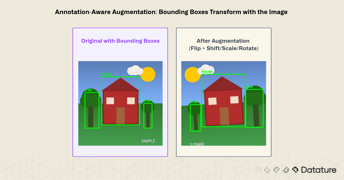

Choosing Augmentations by Task

Not every augmentation works for every task. The table below maps common computer vision tasks to their most effective augmentation strategies:

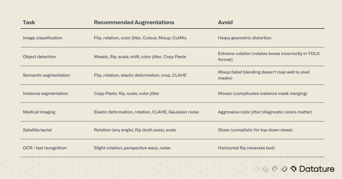
When starting a new project, begin with a conservative pipeline: horizontal flip + small rotation (±10°) + slight brightness/contrast jitter. Measure validation performance, then add techniques one at a time. Monitoring training graphs will show whether each addition helps or hurts.

Common Augmentation Mistakes

1. Augmenting validation and test sets. Augmentation is a training-time technique only. Your validation and test sets should remain unaugmented so that metrics reflect real-world performance. The one exception is test-time augmentation (TTA), which is applied at inference with predictions averaged.

2. Using augmentations that violate label semantics. Flipping a "left turn" sign horizontally creates a "right turn" sign with the wrong label. Rotating digits or letters can change their meaning. Always verify that your chosen transforms preserve the ground truth.

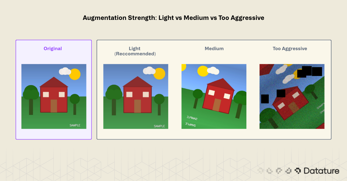
3. Over-augmenting. More is not always better. Stacking too many aggressive transforms produces images so distorted that the model trains on noise. If augmented samples look unrecognizable to a human, they will confuse the model too.

4. Ignoring annotation transforms. Applying geometric augmentation to a detection dataset without transforming bounding boxes creates misaligned annotations. This is one of the most common bugs in custom training pipelines, and it silently degrades mAP. Use a library (Albumentations) that handles this automatically.

5. Applying uniform augmentation to imbalanced classes. If class A has 5,000 images and class B has 500, augmenting both equally maintains the imbalance. Apply stronger or more frequent augmentation to underrepresented classes. See this guide on solving class imbalance for deeper coverage.

Using the Datature Platform for No-Code Augmentation

Not every team wants to write augmentation pipelines from scratch. Datature's Nexus platform includes augmentation as a built-in step in the training workflow, with no code required.

Setting Up Your Dataset

Start by uploading your images to a Nexus project. If you already have annotations (bounding boxes, polygons, or segmentation masks), import them alongside the images. For new datasets, use Nexus's annotation tools: rectangle, polygon, paintbrush, freedraw, and IntelliBrush for AI-assisted labeling.

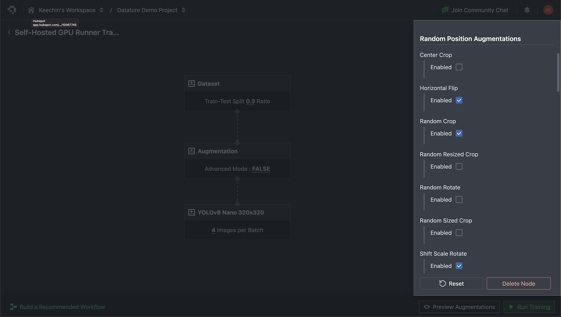
Configuring Augmentations in the Workflow Builder

In the Nexus workflow builder, add an Augmentations node between your dataset and training nodes. The augmentation settings are grouped into two categories:

• Random Position Augmentations: Horizontal flip, vertical flip, rotation, crop, and scaling. Configure probability and range for each.
• Color Space Augmentations: Brightness, contrast, saturation, and hue adjustments. Each has configurable min/max ranges.

Advanced Mode exposes granular control over every parameter. The platform also includes a preview panel that lets you compare augmented images against originals before starting training, so you can verify that transforms look reasonable for your specific dataset.

Training with Augmentation

With augmentation configured, select a model architecture. Nexus supports multiple families including RetinaNet, FasterRCNN, EfficientDet, YOLO variants, MaskRCNN, and DeepLabV3. Augmentations apply automatically during training with no extra configuration.

After training completes, evaluate your model with confusion matrices and training graphs directly in Nexus. Export trained models as TFLite for mobile deployment or standard formats for cloud inference.

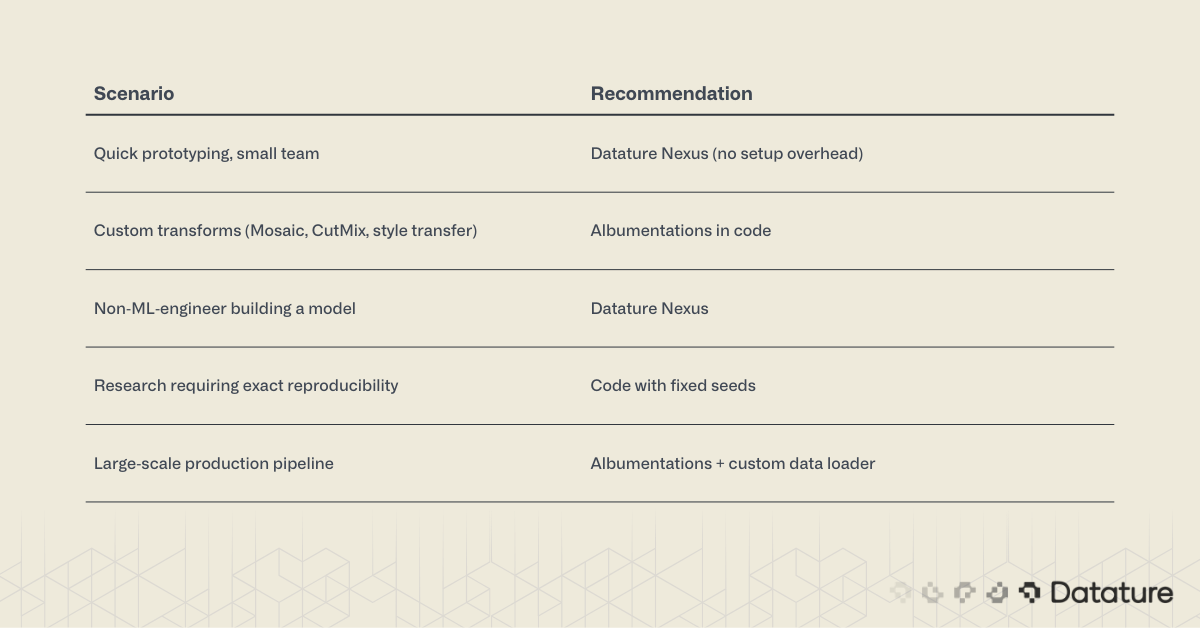
When to Use Platform Augmentation vs. Code

Summary

Image augmentation generates training variety from existing data by applying geometric, color, erasing, and mixing transforms. It reduces overfitting, improves generalization, and costs nothing beyond compute time.

For code-based workflows, Albumentations is the standard: it's fast, supports 70+ transforms, and handles bounding box and mask alignment automatically. Keras ImageDataGenerator works for simple classification projects but lacks the depth needed for detection and segmentation.

For no-code workflows, Datature Nexus includes augmentation as part of its end-to-end pipeline: dataset management, annotation, augmentation, training, and deployment in a single platform.

The key to effective augmentation is matching transforms to your task and deployment conditions. Start simple, measure results with training graphs, and add complexity only when validation metrics improve.