VLM Training Metrics and Loss Functions: A Technical Reference [2026]

Introduction

VLM evaluation is harder than classical computer vision evaluation. Object detection has mAP; segmentation has IoU. Both map directly to spatial accuracy. VLM outputs are free-form text where the same meaning can be expressed in dozens of equally valid ways. This reference covers the ten metrics used to evaluate VLM outputs and the five loss functions used to train them, with formulas first, intuition second, and code throughout.

Evaluation Metrics

VLM evaluation metrics fall into two categories: reference-based metrics that compare model output to human-written ground truth, and reference-free metrics that assess quality directly from the image-text pair. The sections below cover all ten, grouped by approach.

N-gram Metrics

BLEU (Bilingual Evaluation Understudy)

BLEU measures modified n-gram precision between generated and reference text. For n-grams of size 1 through N (typically N=4), it clips n-gram counts to avoid rewarding repetition and applies a brevity penalty for short outputs.

BLEU-N = BP x exp( sum(n=1 to N) w_n x log p_n )
‍p_n = clipped n-gram precision, w_n = 1/N (uniform weight), and BP = min(1, exp(1 - ref_len / gen_len)) is the brevity penalty

Worked Example: BLEU-4 Step by Step

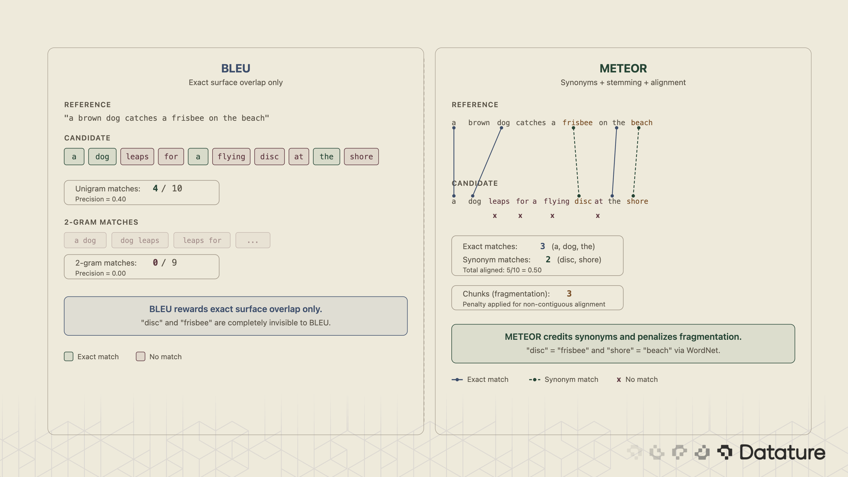
        Reference: "a brown dog catches a frisbee on the beach" (9 tokens)

        Candidate: "a dog leaps for a flying disc at the shore" (10 tokens)

        1-gram matches (clipped): "a" (clipped to 2 of 2 in ref), "dog" (1), "the" (1) = 4 matches / 10 candidate unigrams. p_1 = 0.40‍

        2-gram matches: No candidate bigram appears in the reference. p_2 = 0/9 = 0.0 (requires smoothing)

        3-gram matches: 0/8. p_3 = 0.0 (requires smoothing)

        4-gram matches: 0/7. p_4 = 0.0 (requires smoothing)

        Brevity penalty: ref_len = 9, gen_len = 10, so BP = 1.0 (candidate is longer than reference, no penalty).

Without smoothing, BLEU-4 = 0 because p_2, p_3, and p_4 are all zero. With Method 1 smoothing (adding epsilon to zero counts), BLEU-4 ~ 0.059. This illustrates why BLEU fails on paraphrases: "frisbee"/"disc" and "beach"/"shore" get zero credit.‍

# Prerequisites: pip install nltk==3.9.1
from nltk.translate.bleu_score import sentence_bleu, SmoothingFunction

reference = ["a brown dog catches a frisbee on the beach".split()]
candidate = "a dog leaps for a flying disc at the shore".split()

# BLEU-4 with smoothing (avoids zero scores on short sentences)
smooth = SmoothingFunction().method1
score = sentence_bleu(reference, candidate, weights=(0.25, 0.25, 0.25, 0.25), smoothing_function=smooth)

print(f"BLEU-4: {score:.4f}")
# Expected output: BLEU-4: ~0.059

‍

Strengths: Fast, widely reported, corpus-level scores are more reliable than sentence-level.
‍Weaknesses: Pure precision - ignores recall. No synonym handling. Correlates poorly with human judgment on individual examples.

METEOR (Metric for Evaluation of Translation with Explicit Ordering)

METEOR fixes BLEU's biggest weaknesses. It performs unigram matching with three extensions: exact match, stemming ("running" matches "runs"), and synonym lookup via WordNet. It computes precision P and recall R, combines them with a harmonic mean weighted toward recall (alpha=0.9), then applies a fragmentation penalty.

# Prerequisites: pip install nltk==3.9.1
# First run: nltk.download('wordnet'); nltk.download('omw-1.4')
from nltk.translate.meteor_score import meteor_score

reference = "a brown dog catches a frisbee on the beach".split()
candidate = "a dog leaps for a flying disc at the shore".split()

score = meteor_score([reference], candidate)
print(f"METEOR: {score:.4f}")
# Expected output: METEOR: ~0.29 (higher than BLEU due to synonym matching)

‍

Note: meteor_score expects tokenized word lists, not raw strings. Passing raw strings causes it to split on characters, producing incorrect scores. Always call .split() before passing them in.

ROUGE-L

ROUGE-L computes the longest common subsequence (LCS) between candidate and reference, then derives precision, recall, and F1 from the LCS length. Originally designed for summarization evaluation (Lin, 2004), it's useful for long-form VLM outputs.

# Prerequisites: pip install rouge-score==0.1.2
from rouge_score import rouge_scorer

scorer = rouge_scorer.RougeScorer(['rougeL'], use_stemmer=True)
reference = "a brown dog catches a frisbee on the beach"
candidate = "a dog leaps for a flying disc at the shore"

scores = scorer.score(reference, candidate)
print(f"ROUGE-L F1: {scores['rougeL'].fmeasure:.4f}")
# Expected output: ROUGE-L F1: ~0.3158

‍

Worked Example: ROUGE-L Step by Step

Reference: "a brown dog catches a frisbee on the beach" (9 tokens)

Candidate: "a dog leaps for a flying disc at the shore" (10 tokens)

Step 1: Find the Longest Common Subsequence (LCS)

The LCS is the longest sequence of tokens that appear in both strings in the same order, but not necessarily next to each other. We scan through the candidate and check which tokens also appear in the reference, preserving order.

Working through it token by token:

• "a" - in reference? Yes (position 1). Take it.
• "dog" - in reference after position 1? Yes (position 3). Take it.
• "leaps" - in reference after position 3? No. Skip.
• "for" - in reference after position 3? No. Skip.
• "a" - in reference after position 3? Yes (position 5). Take it.
• "flying" - in reference after position 5? No. Skip.
• "disc" - in reference after position 5? No. Skip.
• "at" - in reference after position 5? No. Skip.
• "the" - in reference after position 5? Yes (position 8). Take it.
• "shore" - in reference after position 8? No. Skip

Step 2: Calculate Precision and Recall

LCS = ["a", "dog", "a", "the"] - length = 4

Precision = 4/10 = 0.400.
Recall = 4/9 = 0.444. F1 = 2 * 0.400 * 0.444 / (0.400 + 0.444) = 0.421

Step 3: Calculate F1

F1 = 2 * P * R / (P + R)
  = 2 * 0.400 * 0.444 / (0.400 + 0.444)
  = 0.3556 / 0.844
  = 0.421

Why does the code output ~0.316 instead of 0.421? The code above sets use_stemmer=True, which reduces tokens to stems before matching. Stemming changes which tokens align - for example, "catches" stems to "catch" and "shore" to "shore" - and the library's internal tokenizer may split tokens differently than simple whitespace splitting. The math above shows the raw LCS process on unstemmed tokens. When you compare your hand calculation to a library's output, always check whether stemming, lowercasing, or tokenization differences explain the gap.

2.2 Captioning Metrics

CIDEr (Consensus-based Image Description Evaluation)

CIDEr applies TF-IDF weighting to n-grams before computing cosine similarity between candidate and reference vectors (Vedantam et al., 2015). Its key insight: n-grams frequent across all images ("on the left side") are less informative than n-grams unique to a particular image ("wearing a red hat"). CIDEr downweights the former through IDF and rewards the latter. This makes it the standard captioning benchmark metric because it captures image-specific content.

Strengths: Designed for captioning. TF-IDF rewards image-specific content. Uses multiple references (consensus). Highest correlation with human judgment among n-gram metrics for captioning. Weaknesses: Requires a reference corpus for IDF statistics. Sensitive to corpus composition. The 0–10 scale (CIDEr-D) isn't intuitive.

# Prerequisites: pip install pycocoevalcap==1.2
from pycocoevalcap.cider.cider import Cider

# Format: {image_id: [caption_string, ...]} for both refs and hypotheses
refs = {0: ["a brown dog catches a frisbee on the beach",
             "a dog playing with a disc on sandy ground"]}
hyps = {0: ["a dog leaps for a flying disc at the shore"]}

cider = Cider()
avg_score, per_image = cider.compute_score(refs, hyps)
print(f"CIDEr: {avg_score:.4f}")
# Expected output: CIDEr: ~0.60 (on a 0-10 scale; note: single-image corpus gives degenerate IDF weights - use 100+ images for reliable scores)

‍

SPICE (Semantic Propositional Image Caption Evaluation)

SPICE parses both candidate and reference into scene graphs - nodes (objects), attributes, and relationships - then computes F1 over the tuples. "A large brown dog on a sandy beach" becomes nodes (dog, beach), attributes (large, brown, sandy), and relations (dog ON beach). Unlike n-gram metrics, SPICE catches semantic inversions: "dog chasing cat" vs. "cat chasing dog" score identically on BLEU but differently on SPICE.

2.3 More Metrics

BERTScore

BERTScore (Zhang et al., 2020) computes token-level cosine similarity using contextual embeddings from a pretrained transformer. Because "dog" and "canine" have near-identical BERT representations, BERTScore handles synonyms far better than any n-gram metric.

# Prerequisites: pip install bert-score==0.3.13 torch==2.2.0
from bert_score import score

refs = ["a brown dog catches a frisbee on the beach"]
cands = ["a dog leaps for a flying disc at the shore"]

# Using roberta-large as the default backbone
P, R, F1 = score(cands, refs, lang="en", verbose=True)
print(f"BERTScore F1: {F1[0]:.4f}")
# Expected output: BERTScore F1: ~0.91 (much higher than BLEU - captures semantic similarity)

CLIPScore

CLIPScore (Hessel et al., 2021) is the only major reference-free metric. It computes cosine similarity between the CLIP image embedding and the CLIP text embedding of the candidate caption. No ground-truth references needed. This makes it uniquely valuable for evaluating outputs when you have the input image but no reference captions.

# Prerequisites: pip install transformers==4.40.0 torch==2.2.0 Pillow==10.3.0
import torch
from transformers import CLIPProcessor, CLIPModel
from PIL import Image

model = CLIPModel.from_pretrained("openai/clip-vit-base-patch32")
processor = CLIPProcessor.from_pretrained("openai/clip-vit-base-patch32")

# Load your image (replace with actual path)
image = Image.open("dog_beach.jpg")
caption = "a dog leaps for a flying disc at the shore"

inputs = processor(text=[caption], images=image, return_tensors="pt", padding=True)
with torch.no_grad():
    outputs = model(**inputs)

# CLIPScore = max(100 * cosine_similarity, 0) per Hessel et al.
# logits_per_image uses a learned temperature (~100) that approximates the *100 scaling
clip_score = max(outputs.logits_per_image.item(), 0)
print(f"CLIPScore: {clip_score:.2f}")
# Expected output: CLIPScore: ~24-28 (scale depends on CLIP model variant)

‍

Strengths: Reference-free. Measures actual image-text alignment. Fast.
‍Weaknesses: Inherits CLIP's biases. Can't catch hallucinated details that happen to be plausible. Coarse - doesn't capture fine-grained factual accuracy.

2.4 Task-Specific Metrics

VQA Accuracy

The VQA metric (Antol et al., 2015) accounts for inter-annotator disagreement: min(count(model_answer) / 3, 1). If 3+ annotators gave the same answer, accuracy = 1.0. If 1 annotator agreed, accuracy = 0.33. Use only when multi-annotator reference answers exist; for single-reference VQA, use Exact Match or BERTScore.

Exact Match and F1

For structured VLM outputs - invoice field extraction, document QA, bounding box coordinates as text - Exact Match is binary and token-level F1 gives partial credit.

ANLS (Average Normalized Levenshtein Similarity)

ANLS is the standard metric for document understanding (DocVQA, InfoVQA, ST-VQA). It computes normalized edit distance between predicted and reference strings, giving partial credit for near-correct OCR outputs.

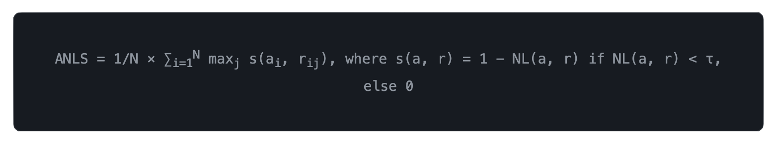
NL(a, r) is the normalized Levenshtein distance (edit distance / max length). τ is typically 0.5, meaning predictions within 50% edit distance get partial credit, while completely wrong answers score zero.

2.5 Metrics-by-Task Quick Reference

3. Loss Functions for Fine-Tuning

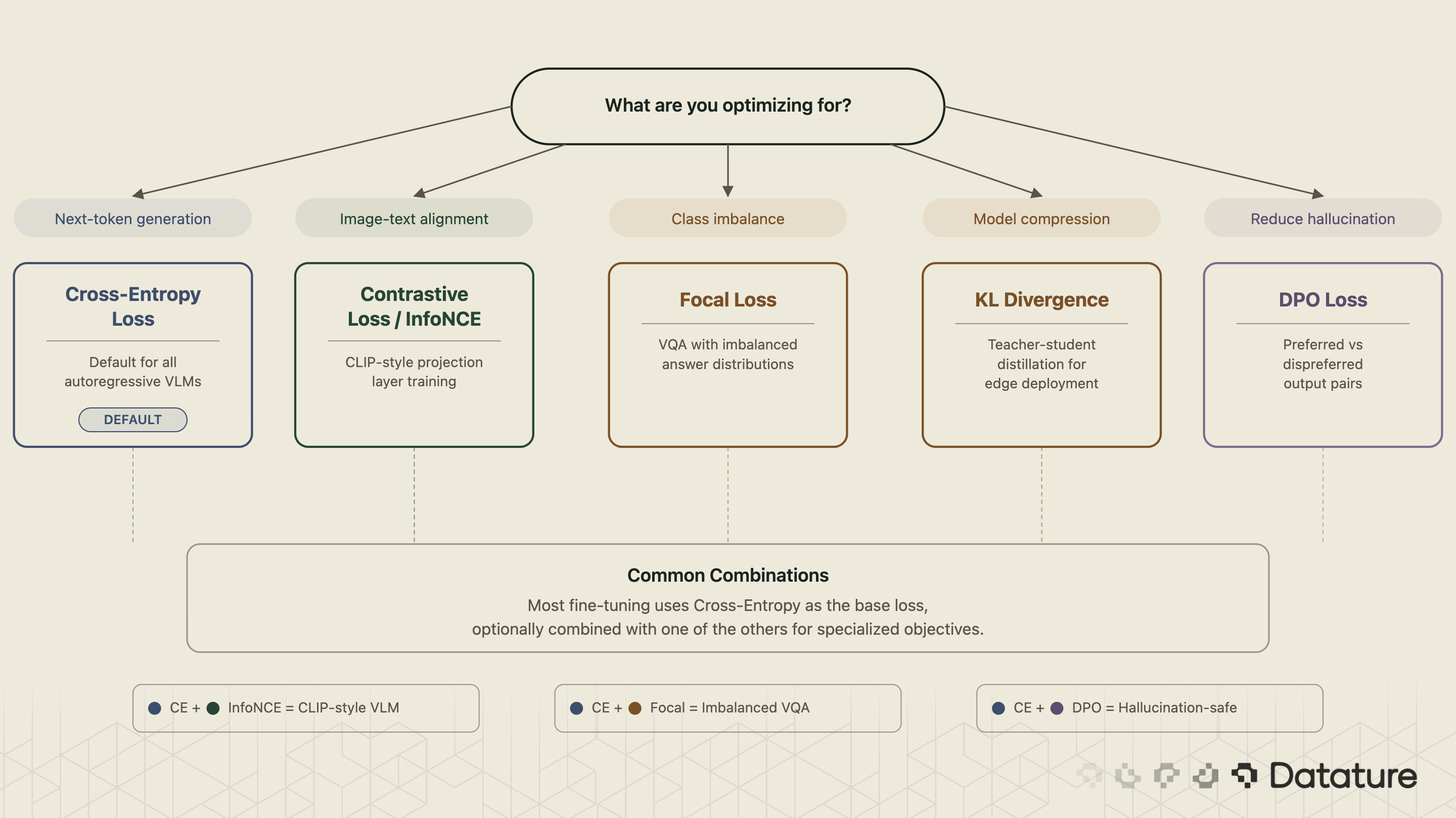
Evaluation metrics tell you how good a model is. Loss functions tell the model how to improve. They aren't interchangeable: CIDEr and BLEU aren't differentiable and can't be used as training losses directly. This section covers the loss functions used in VLM fine-tuning, ordered by how commonly they appear.

3.1 Cross-Entropy Loss

The foundation of all autoregressive VLMs. Measures how well the model predicts the next token given all previous tokens and the image.

During fine-tuning, restrict loss computation to response tokens only (mask prompt/instruction tokens with -100). If you're fine-tuning PaLIGemma or fine-tuning Qwen2.5-VL, this is the loss you're optimizing.

3.2 Contrastive Loss (InfoNCE)

Trains the model to produce similar embeddings for matching image-text pairs and dissimilar embeddings for non-matching pairs.

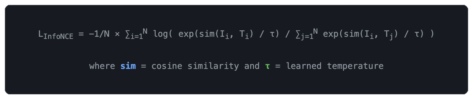
When to Use? Fine-tuning the vision-language alignment stage (the projection layer between vision encoder and LLM). Also used in retrieval-augmented VLMs where image-text matching is critical.

3.3 Focal Loss

Focal loss (Lin et al., 2017, "Focal Loss for Dense Object Detection") modifies cross-entropy to downweight easy examples and focus on hard ones. It adds a modulating factor (1 - p_t)^γ where γ typically ranges from 1 to 3. In VQA, trivially easy questions ("Is this a photo?" → "yes") dominate the loss unless downweighted.

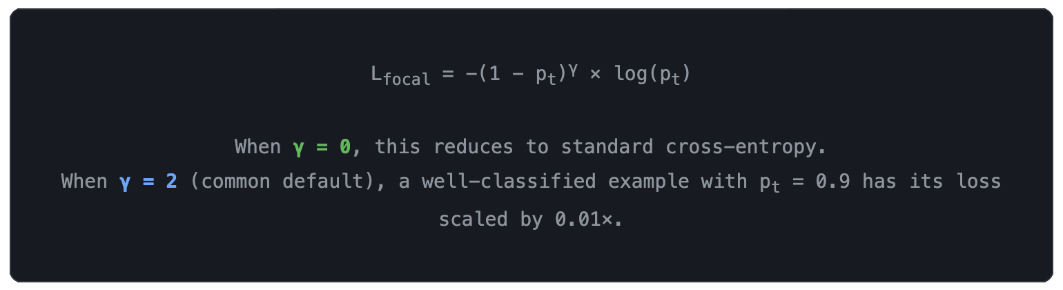
When to Use: VQA fine-tuning with class imbalance (many "yes/no" examples, few detailed answers). Also useful when combining VQA with classification objectives.

3.4 KL Divergence (Distillation)

Knowledge distillation trains a smaller "student" VLM to match the output distribution of a larger "teacher." KL divergence measures the difference between the two probability distributions. The total loss is ↘

When to use: Compressing a large VLM into a deployable size. Teams deploying to edge devices like Raspberry Pi or using post-training quantization often start with distilled models.

3.5 DPO / RLHF Loss

Direct Preference Optimization (DPO) has largely replaced the more complex RLHF pipeline for VLM preference tuning. DPO optimizes directly on pairs of preferred (y_w) and dispreferred (y_l) outputs without a separate reward model.

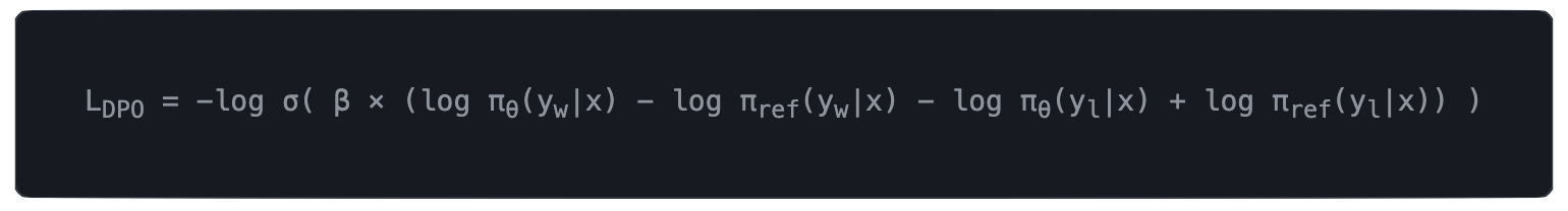
When to use: Reducing hallucination. Particularly effective for visual question answering tasks. RLHF remains one of the most consistently requested feature on Datature Vi, and we will be working on an interface for enabling teams to quickly build their own DPO workflow.

‍

3.6 Training Loop (PyTorch + W&B)

A simplified PyTorch training loop showing how cross-entropy loss and validation metrics fit together.

# Prerequisites: pip install torch==2.2.0 transformers==4.40.0 wandb==0.16.0
import torch
import wandb
from torch.nn import CrossEntropyLoss
# from transformers import CLIPModel, CLIPProcessor  # used in compute_clipscore()

# Initialize logging
wandb.init(project="vlm-finetune", config={"lr": 2e-5, "epochs": 3})

loss_fn = CrossEntropyLoss(ignore_index=-100)  # -100 masks prompt tokens

# Simplified training step (pseudocode for structure, not runnable as-is)
for epoch in range(num_epochs):
    model.train()
    for batch in train_loader:
        images, input_ids, labels = batch
        outputs = model(images=images, input_ids=input_ids)

        # Cross-entropy loss on response tokens only (labels have -100 for prompt)
        loss = loss_fn(outputs.logits.view(-1, vocab_size), labels.view(-1))
        loss.backward()
        optimizer.step()
        optimizer.zero_grad()

        wandb.log({"train/loss": loss.item(), "train/lr": optimizer.param_groups[0]["lr"]})

    # Validation: compute CIDEr and CLIPScore on held-out set
    model.eval()
    with torch.no_grad():
        val_clip_scores, val_cider_scores = [], []
        for val_batch in val_loader:
            generated = model.generate(val_batch["images"], max_new_tokens=64)
            # compute_clipscore() and compute_cider() are your metric functions
            val_clip_scores.append(compute_clipscore(val_batch["images"], generated))
            val_cider_scores.append(compute_cider(generated, val_batch["references"]))

    wandb.log({
        "val/clipscore": sum(val_clip_scores) / len(val_clip_scores),
        "val/cider": sum(val_cider_scores) / len(val_cider_scores),
    })

# Expected: loss decreases over epochs; CLIPScore and CIDEr increase on val set

‍

Common Pitfall - Don't use CIDEr or BLEU as a training loss. These metrics aren't differentiable (they involve argmax over discrete tokens). Use cross-entropy for training and n-gram/neural metrics for evaluation only. The exception is SCST (Self-Critical Sequence Training), which uses CIDEr as a reward signal through a policy gradient estimator.

4. Choosing the Right Metric

Start with the task. Captioning systems should report CIDEr as the primary benchmark metric and CLIPScore for reference-free evaluation. VQA tasks with multi-annotator data use VQA Accuracy. Document understanding tasks use ANLS.

In all cases, report at least two metrics because no single number captures VLM quality. For spatial evaluation metrics like mAP and IoU, see our guide on evaluating CV models with confusion matrices.

5. Further Reading

The original papers behind each metric, ordered chronologically:

• BLEU - Papineni, K., Roukos, S., Ward, T., & Zhu, W. (2002). "BLEU: a Method for Automatic Evaluation of Machine Translation." Proceedings of ACL 2002. ACL Anthology
• ROUGE - Lin, C.-Y. (2004). "ROUGE: A Package for Automatic Evaluation of Summaries." Text Summarization Branches Out, ACL 2004. ACL Anthology
• METEOR - Banerjee, S. & Lavie, A. (2005). "METEOR: An Automatic Metric for MT Evaluation with Improved Correlation with Human Judgments." ACL Workshop 2005. ACL Anthology
• CIDEr - Vedantam, R., Zitnick, C.L., & Parikh, D. (2015). "CIDEr: Consensus-based Image Description Evaluation." CVPR 2015. arXiv: 1411.5726
• VQA - Antol, S. et al. (2015). "VQA: Visual Question Answering." ICCV 2015. arXiv: 1505.00468
• SPICE - Anderson, P., Fernando, B., Johnson, M., & Gould, S. (2016). "SPICE: Semantic Propositional Image Caption Evaluation." ECCV 2016. arXiv: 1607.08822
• BERTScore - Zhang, T., Kishore, V., Wu, F., Weinberger, K.Q., & Artzi, Y. (2020). "BERTScore: Evaluating Text Generation with BERT." ICLR 2020. arXiv: 1904.09675
• CLIPScore - Hessel, J., Holtzman, A., Forbes, M., Le Bras, R., & Choi, Y. (2021). "CLIPScore: A Reference-free Evaluation Metric for Image Captioning." EMNLP 2021. arXiv: 2104.08718

‍

6. Frequently Asked Questions

What is The Best Single Metric for Evaluating Image Captions?

CIDEr, because its TF-IDF weighting rewards image-specific content over generic descriptions and it has the highest correlation with human judgment among n-gram metrics. For systems without ground-truth references, CLIPScore is the practical alternative.

Which Loss Function Should I Start with for VLM Fine-Tuning?

Cross-entropy loss on response tokens (masking prompt tokens with -100). This is the default for every autoregressive VLM. Add contrastive loss if you need better image-text alignment, or DPO loss if you have preference data and want to reduce hallucination.

Can I Use CIDEr or BLEU as a Training Loss?

No. Both metrics involve argmax over discrete tokens and aren't differentiable. Use cross-entropy for training and n-gram/neural metrics for evaluation only. The exception is reinforcement learning approaches like SCST that use CIDEr as a reward signal through a policy gradient estimator.

What is ANLS and When Should I Use It?

ANLS (Average Normalized Levenshtein Similarity) computes normalized edit distance between predicted and reference strings, giving partial credit for near-correct outputs. It's the standard metric for document understanding benchmarks (DocVQA, InfoVQA, ST-VQA) because it tolerates minor OCR errors that would fail Exact Match.

How Can I Get Started with VLMs?

Datature's Vi Platform supports the structured annotation workflows needed to build high-quality VLM training datasets - from image-text pairs for captioning to multi-attribute labels for VQA - with active learning to prioritize which images to annotate next.